A full wave description for thin wire structures with TLST and perturbation theory

(1)

https://doi.org/10.5194/ars-16-123-2018

A full wave description for thin wire structures with TLST and

perturbation theory

Fabian Ossevorth, Ralf T. Jacobs, and Hans Georg Krauthäuser

Technische Universität Dresden, Elektrotechnisches Institut, Theoretische Elektrotechnik & EMV, 01062 Dresden, Germany Correspondence:Fabian Ossevorth ([email protected])

Received: 28 January 2018 – Revised: 30 April 2018 – Accepted: 26 June 2018 – Published: 4 September 2018

Abstract. A full wave description of a thin wire structure, that includes mutual interactions and radiation, can be ob-tained in closed form with the so-called Transmission Line Super Theory or a refined variant of this method that utilises perturbation theory. In either procedure, a set of mixed po-tential integral equations is solved for the currents that prop-agate along a wire. With the perturbation approach, no itera-tion is required to approximate the initial current distribuitera-tion on the wire. This procedure will be applied to solve multi-wire problems. The theory will be derived and computed re-sults will be shown to be in good agreement with method of moment computations.

1 Introduction

The solution to electromagnetic compatibility problems be-comes more challenging if a large number of electronic de-vices or modules of a system is placed in a confined space. Mutual interactions and especially mutual coupling between wires connecting individual modules might occur, which can lead to malfunctions and undesired system conditions. In or-der to circumvent erratic system performance, an accurate estimation of the coupling parameters is necessary.

The Transmission Line Super Theory (TLST) is an iter-ative procedure (Nitsch et al., 2009), where the wire pa-rameters like the inductance and capacitance per unit length are first determined under the assumption to be dependent upon position only. Frequency dependence is accounted for in the subsequent iterations. With these parameters, a sys-tem of ordinary differential equations of first order with vari-able coefficients is established and solved for the unknown currents with the aid of a matrizant, but the solution of the resulting system of equations is computationally extensive.

A perturbation approach for the TLST was formulated in Nitsch and Tkachenko (2010).

In the perturbation method, the currents to be deter-mined are initially approximated with values calculated us-ing the conventional transmission line theory. These cur-rents are subsequently employed to compute the parameters of the wire structure using mixed potential integral equa-tions (MPIE). The parameters are then used in a system of ordinary differential equations similar to the TLST to as-certain the currents on the wires. In contrast to the TLST, it is not necessary in the perturbation method to determine the wire parameters in a first iteration, which therefore re-quires less computation time. The theoretical formulation of the perturbation approach in Nitsch and Tkachenko (2010) provides the basis for this investigation. The procedure will be derived and applied to the solution of multi-wire prob-lems. Section 2 facilitates essential background theory. The TLST is described in Sect. 3 where a detailed derivation of the perturbation theory is given in Sect. 3.2. Simulated re-sults are shown in Sect. 4 which are validated by comparison with method of moment computations.

2 Background theory

The TLST is based on the solution of the Helmholtz equa-tions

1A+k2A= −µJs (1)

and

1φ+k2φ= −%

ε. (2)

(2)

charge density. The wave numberkis given by

k=ω√µε. (3)

where µ is the permeability and ε the permittivity of the medium. For sources above a perfectly conducting ground plane, the two potentials are determined by

A(r)= µ

4π

Z Z Z

D

Js(r0)e

−j k|r−r0_|

|r−r0_|

+Js₁(r01)

e−j k|r−r01| |r−r0

1|

dτD (4)

and φ(r)= 1

4π ε

Z Z Z

D %(r0)e

−j k|r−r0_|

|r−r0_|

−%(r01)

e−j k|r−r01| |r−r0

1|

dτD. (5)

r represents the vector to the field point,r0the vector to the source point,r01the vector to the image of the source point,

andJs₁(r01)the image current density.Dis the source

vol-ume and dτDa volume element.

The electric field is given by the sum of the scattered field and the exciting or incident field,

E(r)=Escat(r)+Einc(r). (6)

The scattered field is given by

Escat(r)= −j ωA(r)−gradφ(r). (7) The electric field and the potentials on the surfaceS of the source volume are related through the boundary conditions

E(r)·et(r)

S= 1 ~J

s₍_r₎_·_e t(r)

S

=Escat(r)·et(r)

_S+Einc(r)·et(r)

S (8)

and 1 ~J

s₍_r₎_·_e t(r)

S= −j ωA(r)·et(r)

S

−gradφ(r)·et(r)

_S+E

inc₍_r₎_·_e

t(r)

_S. (9)

Applying the thin wire approximation (Nitsch et al., 2009), where the current is concentrated on the axis of the wire which possesses a small radius a (Nitsch and Tkachenko, 2010), and substituting of Eqs. (4) and (5) into Eq. (9) leads to

j ω µ 4π

L

Z

0

G_A(l, l0)Is(l0)dl0+ 1

4π ε ∂ ∂l

L

Z

0

λ(l0)G_φ(l, l0)dl0

− 1

C0

c

∂

∂lλ(l)+Z 0

Is(l)=Einc(r)·et(r), (10) where Is represents the current in the wire and λthe line charge density.G_AandG_φdenote the Green’s functions for

the potentials, given by

G_A(l, l0)=e

−j k|r(l)−r0(l0)|

|r(l)−r0_(l0₎_|et(l)·et(l 0₎

−e

−j k|r(l)−r0

1(l0)|

|r(l)−r0

1(l0)|

et(l)·et1(l

0

), (11)

G_φ(l, l0)=e

−j k|r(l)−r0_(l0_)|

|r(l)−r0_(l0₎_| −

e−j k|r(l)−r01(l0)| |r(l)−r0

1(l0)|

. (12)

In case of a lossy conductor in the thin wire approximation, the tangentialE-field becomes

1 ~J

s₍_r₎_·_e t(r)

_S=Z

0

Is(l), (13)

with the impedance per unit length Z0= − Zc

2π a I0(γ a)

I1(γ a)

(14)

evaluated on the surface of the wire (Nitsch and Tkachenko, 2006; Tesche et al., 1997). The characteristic impedanceZ_c is

Z_c= s

j ωµ

~+j ωε. (15)

For a dielectrically coated wire an additional capacitanceC_c0 needs to be considered in Eq. (10), which is given by C_c0=2π ε

lnb_a εc

εc−1

. (16)

An alternative formulation to Eq. (10) can be established by substituting Eq. (4) in Eq. (9), which yields

∂ φ ∂l +j ω

µ 4π

L

Z

0

G_A(l, l0)Is(l0)dl0+Z0Is(l)

=Einc(r)·et(r). (17)

Employing the continuity conditionλ= − 1

j ωIs in conjunc-tion with the thin wire approximaconjunc-tion in Eq. (5) leads to

φ(l)+ 1

j ω4π ε L

Z

0

G_φ(l, l0)∂I s_(l0₎ ∂l0 dl

0

− 1

j ωC0

c

∂Is(l)

∂l =0. (18)

(3)

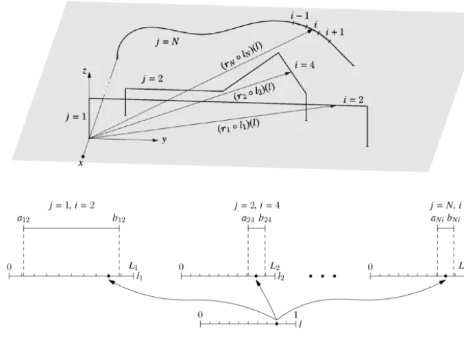
Figure 1.Point on wirejand segmentias function of the global parameterl, shown forl=0.8.

3 Full-wave transmission line theory

In order to solve multi-wire problems, a single parameter is required to simultaneously reference points on all the wires. This can be achieved with the mapping

lj=lLj with 0≤l≤1, (19)

on wirej of lengthLj withj=1, . . ., N, whereN denotes the number of wires.lj is a curve length parameter for wire j that depends on the single global parameterl. Figure 1 de-picts an example withN wires. Each wire is divided into a number of segments. Arbitrarily curved wires are linearized, so that each segment is straight. The number of segments on a particular wire is as a result dependent on the curvature of the wire. In terms of the curve length parameter lj, a seg-ment i of wire j extends from aj i tobj i, as shown in the figure for three different segments. The linearization leads to a constant tangent vector on a segment. This simplifies the integration considerably, so that Eq. (10) can be written as

j ω µ 4π

N

X

p=1 1 Z

0

LjGA,jp(lLj, l0Lp)Isp(l 0

Lp)Lpdl0

+ 1

4π ε ∂ ∂l

N

X

p=1 1 Z

0

LpGφ,jp(lLj, l0Lp)λpdl 0

+ 1

C0

c

∂

∂lλj(lLj)+Z 0

jLjIsj(lLj)

=LjEincj ·et,j(rj). (20)

Equivalently, for Eqs. (17) and (18) it follows ∂ φ

j(l) ∂l +j ω

µ 4πLj

N

X

p=1 1 Z

0

G_A,jp(lLj, l0Lp)I_p(l0Lp)Lpdl0

+Z0_jLjIsj(lLj)=LjEincj ·et(rj) (21) and

φ j(l)+

1 j ω4π ε

N

X

p=1 1 Z

0

G_φ,jp(lLj, l0Lp)∂I s p(l

0₎ ∂l0 dl

0

− 1

j ωC0

cLj

∂Is_j(lLj)

∂l =0. (22)

Alternative parameterizations to Eq. (19) are possible (Nitsch and Tkachenko, 2010), they lead to the same solutions but with slightly different expressions for the entries of the pa-rameter matrices.

3.1 Transmission Line Super Theory

In this section Eq. (20) is solved iteratively using Transmis-sion Line Super Theory (Haase, 2005) with a frequency inde-pendent current. Since a transmission line is characterized by the parametersP, the unknown quantities have to be deter-mined before computing the currents. By casting the MPIE into matrix form, a position dependent differential equation system of the form

d dl

φ(l) I (l)

+j ωP(l)

φ(l0)

I (l0)

=

φinc(l) Iinc(l)

(4)

can be established. The parametersP will be determined it-eratively, where Eq. (23) is solved using a product integral (Gantmacher, 1960; Dollard and Friedman, 1984). Rewriting Eq. (20) in this form leads to

j ω1 1_∂l∂

1 Z

0

K_L(l, l0, k) 0 0 K_C(l, l0, k)

I(l0)

λ(l0)

dl0

+C0−1 c λ+Z

0_I₌₀ ₍₂₄₎

with

K_L(l, l0, k)= µ

4πdiag Lj

G_A(l, l0, k), (25)

K_C(l, l0, k)= 1

4π εGφ(l, l 0

, k). (26)

The wires are excited at their terminals, which are located outside the source volume and the influence of external fields is neglected. The matrices G_A(l, l0, k) and G_φ(l, l0, k) are given by

G_A(l, l0, k)=G_A,jp(lLj, l0Lp)Lp,

j =1,2, . . ., N;p=1,2, . . ., N (27) and

G_φ(l, l0, k)=G_φ,jp(lLj, l0Lp, )

j =1,2, . . ., N;p=1,2, . . ., N. (28) Each matrix has the dimensionN×N, whereN represents the number of wires. The impedance and capacitance matri-ces have diagonal form and are given by

Z0₌_diag _L jdiag

Z0_j,forj=1, . . ., N, (29)

C0

c=diag Ljdiag

C_c0_,j,forj =1, . . ., N. (30) Under the assumption that the line charge and current are determined by the solution of a differential equation sys-tem (23), the solution is of the form

I(l0)

λ(l0)

=e

l0

l(−j ωP)

I(l)

λ(l)

. (31)

e l

0

l denotes the propagator, which is also referred to as ma-trizant. Employing Eq. (31) in Eq. (24) leads to

j ω1 1_∂l∂

1 Z

0

K_L(l, l0, k) 0 0 K_C(l, l0, k)

e l

0 l

I(l)

λ(l)

dl0

+C0−_c 1λ+Z0I=0, (32)

which can be written as

j ω1 1_∂l∂

R₁₁(l, k)I(l)+R₁₂(l, k)λ(l)

R₂₁(l, k)I(l)+R₂₂(l, k)λ(l)

+C0−1 c λ+Z

0_I₌₀ ₍₃₃₎

where the submatricesR_ij contain the solutions of the in-tegrals. Applying the product rule of differentiation, a more compact expression in terms of current and charge can be found if the equation of continuity is applied,

R₂₁ R₂₂

1 0

∂ ∂lI(l)

∂ ∂lλ(l)

+j ω

R₁₁+ 1

j ω ∂

∂lR21+Z 0

R₁₂+ 1

j ω ∂

∂lR22+C0−1c

0 1

I(l)

λ(l)

=0. (34)

This can be rearranged as ∂

∂l

I(l)

λ(l)

+j ωP_iq(l)

I(l)

λ(l)

=

0 0

, (35)

which is a differential equation system for current and line charge. The parameter matrix P_iq(l, k) follows from Eqs. (34) and (35),

Piq(l, k)=

R₂₁ R₂₂

1 0

−1

R₁₁+ 1 j ω

∂

∂lR21+Z 0

R₁₂+ 1 j ω

∂ ∂lR22+C

0−1 c

0 1

. (36) The submatricesR_ij matrices are unknown and have to be determined in order to obtain the parameters of the transmis-sion line system. Assuming that the matrizant is known, the integral over the Green’s functions can be solved and the sub-matrices can be obtained from Eq. (32), and combined in a matrixRof the form

R=

R₁₁ R₁₂ R₂₁ R₂₂

= 1 Z

0

K_L(l, l0, k) 0 0 K_C(l, l0, k)

e l

0 ldl

0_. ₍₃₇₎

At this point the iteration is started. The identity matrix is used as a first approximation for the matrizant. Assuming the Green’s functions initially to be independent of frequency, allows integrals to be solved analytically (Nitsch et al., 2009). The initial values are then

R(0)₌

1 Z

0

K_L(l, l0) 0 0 K_C(l, l0)

k=0

dl0. (38)

(5)

recasted in a form of a matrizant as written in Eq. (31). The next iteration is performed with the updated matrizant. The iteration matrix at stepncan now be compactly expressed as

R(n)₌

         

        

1 R

0

K_L(l, l0) 0 0 K_C(l, l0)

_k₌₀

dl0_, n=0

1 R

0

K_L(l, l0, k) 0 0 K_C(l, l0, k)

e

l

0

0(−j ωP

(n−1)

iq )dl

0_,

otherwise.

(39)

Usually, the first iteration already delivers accurate results (Haase, 2005). In order to solve the differential equations, boundary conditions are required for current and line charge, which is a non-trivial problem for the charge. In order to cir-cumvent this problem, a potential and current representation is employed. From Eq. (33) it follows

φ=R₂₁I+R₂₂λ, (40)

from which parametersP?_{can be computed, (Haase, 2005),}

P?=

P?₁₁ P?₁₂ P?₂₁ P?₂₂

, (41)

where

P?₁₁=

R₁₂+ 1

j ωC 0

c

−1

R−₂₂1

P?₁₂=R₁₁+ 1

j ω

Z0−C0_c−1R−₂₂1R₂₁−R₁₂R−₂₂1R₂₁ P?

21=R

−1 22

P?₂₂= −R−₂₂1R₂₁

The iterative approach is based on the computation of R, which is then used in Eq. (41). Solving the differential equa-tion in potential-current representaequa-tion leads to the desired result (Rambousky et al., 2013; Rambousky, 2014). The it-erative procedure is expensive in terms of computation time. If a low frequency solution is desired, it is usually sufficient to only use the starting values which then lead to position-dependent parameters. No further iteration is required.R₁₁

and R₂₂ are calculated using Eq. (38) and then used in Eq. (41), which leads to

P?(0)₌ j ω1C 0−1

c R

−1

22 R11+j ω1Z 0

R−₂₂1 0

!

. (42)

An alternative and more efficient method is presented in Sect. 3.2.

3.2 Solution using perturbation theory

The method is based on the direct approximation of the cur-rent on a wire. The procedure will initially be described for a single wire and afterwards be extended to multi-wire ar-rangements. The wire is excited by applying delta sources at

one or both ends of the wire. This leads to two linear inde-pendent solutions for the potential and the current,

φ(l)=C1φ₁(l)+C2φ₂(l) (43)

and

I (l)=C1I1(l)+C2I2(l), (44)

from which the system of ordinary differential equations (ODEs)

∂ ∂l

φ I

+j ω

P₁₁(l) P₁₂(l) P₂₁(l) P₂₂(l)

φ I

=

0 0

, (45)

can be established (Burg et al., 2013; Heuser, 1995). The entriesP_ij are continuously differentiable functions for all l∈ [0,1]. Employing Eqs. (43) and (44) in Eq. (45), leads to

∂ ∂l

φ

1 φ2

I₁ I₂

+j ω

P₁₁(l) P₁₂(l) P₂₁(l) P₂₂(l)

φ

1 φ2

I₁ I₂

=

0 0 0 0

. (46)

The coefficientsP_ijcan now be determined as

P₁₁(l) P₁₂(l) P₂₁(l) P₂₂(l)

= − 1

j ω

∂ ∂lφ1

∂ ∂lφ2

∂

∂lI1 ∂l∂I2

φ

1 φ2

I₁ I₂

−1

, (47)

under the assumption that the Wronskian exists on the entire domain, i.e. for 0≤l≤1. For a multi-wire problem withN wires, Eq. (45) can be written as

∂ ∂l

φ I

+j ω

P₁₁(l) P₁₂(l)

P₂₁(l) P₂₂(l)

φ I

=

0 0

. (48)

The submatricesP_ijare of dimensionN×N, so that the sys-tem Eq. (48) is of dimension 2N×2N. In order to compute the coefficients, the derivatives of the currents are required. These are initially approximated using the theory of travel-ling waves,

I(₁0)=C_I,₁e−j klL, (49) I(₂0)=C_I,₂ej klL. (50) Equation (47) can be generalized forN wires as



 φ

1 φ2

I(₁0) I(₂0) 

=





F_φ,₁ F_φ,₂

diag e−j klLj _diag _ej klLj 



diag C_I,₁ 0 0 diag C_I,₂

(6)

with

F_φ,₁=       f

φ,1,11 fφ,1,12 . . . fφ,1,1N f

φ,1,21 fφ,1,22 . . . fφ,1,2N ..

. ... . .. ...

f

φ,1,N1 fφ,1,N2 . . . fφ,1,N N

      and

F_φ,₂=       f

φ,2,11 fφ,2,12 . . . fφ,2,1N f

φ,2,21 fφ,2,22 . . . fφ,2,2N ..

. ... . .. ...

f

φ,2,N1 fφ,2,N2 . . . fφ,2,N N

      , (52)

where the entries of the matrices are defined as

f

φ,m,jp= Lp

c

(−1)m−1 C_m,jp +

(−1)m cC0

c

e(−1)mj klLj

=(−1)

m−1_L

p 4π εc Np X i=1 bi Z ai

e−j k|rj(lLj)−r0pi(l0Lp)| |rj(lLj)−r0pi(l0Lp)|

−e

−j k|rj(lLj)−r01,pi(l0Lp)|

|rj(lLj)−r01,pi(l0Lp)|

!

e(−1)mj kl0Lp_dl0

+(−1)

m

cC0

c

e(−1)mj klLj ₍₅₃₎

for j, p=1,2, . . ., N. Np denotes the number of segments on wirep,m=1 corresponds to the forward travelling wave andm=2 to the backward travelling wave, whereasC_m,jp refers to the local capacitance between wiresj andp,

C_m,jp=4π ε

  Np X i=1 bi Z ai

−e

−j k|rj(lLj)−r01,pi(l0Lp)|

|rj(lLj)−r01,pi(l0Lp)|

!

e(−1)mj kl0Lp_dl0 !−1

. (54)

The matrix containing the derivatives can be established sim-ilarly,





∂ ∂lφ₁

∂ ∂lφ₂

∂ ∂lI

(0)

1

∂ ∂lI

(0)

2 

=





G_φ,₁ Gφ,2

−j kdiag Lje−j klLj j kdiag Ljej klLj





diag CI,1

0 0 diag CI,2

, (55)

where the elements of the submatrices G_φ,₁ and G_φ,₂ are given by

g

φ,m,jp= −j ωLm,jp−Z

0

Lje(−1) m_{j klL}

j

= −j ωµ 4πLj

Np X

i=1

bi Z

ai

et,j(lLj)

̹_{→ ∞} L3 L2 L1 n P0

P1 P2

P3

Figure 2.Single wire above ground plane.

·et,p(l0Lp)−

e−j k|rj(lLj)−r01,pi(l0Lp)| |rj(lLj)−r01,pi(l0Lp)|

et,j(lLj)

·et1,pi(l

0

Lp)

e(−1)mj kl0Lp_L

pdl0−Z0Lje(−1) m_{j klL}

j_. ₍₅₆₎

The local inductance between wiresj andpis denoted with L_m,jpand given by

L_m,jp= µ

4πLj Np X i=1 bi Z ai

_e−j k|rj(lLj)−r0pi(l0Lp)| |rj(lLj)−r0pi(l0Lp)|

et,j(lLj)

·et,p(l0Lp)−

e−j k|rj(lLj)−r01,pi(l0Lp)| |rj(lLj)−r01,pi(l0Lp)|

et,j(lLj)

·et1,pi(l 0

Lp)

e(−1)mj kl0Lp_L

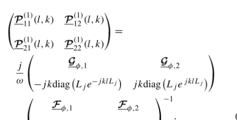
pdl0. (57) The parameter matrix for theN wire problem can as a result be written as





P(₁₁1)(l, k) P(₁₂1)(l, k)

P(₂₁1)(l, k) P(₂₂1)(l, k)

 = j ω  

G_φ,₁ G_φ,₂

−j kdiag Lje−j klLj j kdiag Ljej klLj









F_φ,₁ F_φ,₂

diag e−j klLj _diag _ej klLj 



−1

. (58)

Rewriting the inverse of Eq. (58) following (Bernstein, 2009), allows the parameter matrix to be expressed as

P(₁₁1)(l)= 1

j ω

G_φ,₁D2+−G_φ,₂

F_φ,₂−G_φ,₁D2+

−1

, (59)

P(₁₂1)(l)= 1

j ω

G_φ,₁F−_φ,1₁G_φ,₂−F_φ,₂

D₊−D₋F−_φ,1₁F_φ,₂−1, (60)

P(₂₁1)(l)= −2

cdiag Lj

D₊F_φ,₂−F_φ,₁D2

+

−1

(7)

-10 -8 -6 -4 -2 0 2 4 6 8 10

Re

{ ¯

I

(

l

=

0

)}

in

m

A

Terminal 1

TLST/PT MoM

-5 -4 -3 -2 -1 0 1 2 3 4 5

Im

{ ¯

I

(

l

=

0

)}

in

m

A

0 0.5 1 1.5 2

fin GHz

TLST/PT MoM

-10 -8 -6 -4 -2 0 2 4 6 8 10

Re

{ ¯

I

(

l

=

1

)}

in

m

A

Terminal 2

TLST/PT MoM

-5 -4 -3 -2 -1 0 1 2 3 4 5

Im

{ ¯

I

(

l

=

1

)}

in

m

A

0 0.5 1 1.5 2

fin GHz

TLST/PT MoM

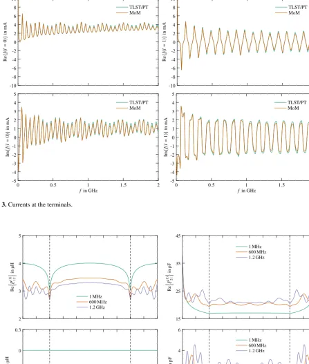
Figure 3.Currents at the terminals.

2 3 4 5

Re

n

¯

P

(

1

)

12

o

in

µH

1 MHz 600 MHz 1.2 GHz

-0.9 -0.6 -0.3 0 0.3

Im

n

¯

P

(

1

)

12

o

in

µH

0 0.1 0.2 0.3 0.4 0.5 0.6 0.7 0.8 0.9 1

l

15 25 35 45

Re

n

¯

P

(

1

)

21

o

in

pF

-2 0 2 4 6

Im

n

¯

P

(

1

)

21

o

in

pF

0 0.1 0.2 0.3 0.4 0.5 0.6 0.7 0.8 0.9 1

l

(8)

-10 -8 -6 -4 -2 0 2 4 6 8 10

Re

{ ¯

I

(

l

=

0

)}

in

m

A

Terminal 1

TLST/PT TLST-0

-6 -5 -4 -3 -2 -1 0 1 2 3 4 5

Im

{ ¯

I

(

l

=

0

)}

in

m

A

0 10 20 30 40 50

fin MHz

TLST/PT TLST-0

-10 -8 -6 -4 -2 0 2 4 6 8 10

Re

{ ¯

I

(

l

=

1

)}

in

m

A

Terminal 2

TLST/PT TLST-0

-6 -5 -4 -3 -2 -1 0 1 2 3 4 5

Im

{ ¯

I

(

l

=

1

)}

in

m

A

0 10 20 30 40 50

fin MHz

TLST/PT TLST-0

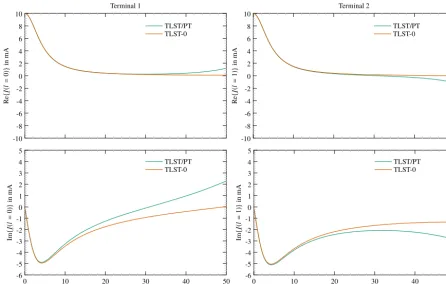
Figure 5.Currents at the terminals in the frequency range from 1 to 50 MHz.

P(₂₂1)(l)= −1

cdiag Lj

D₋F−1

φ,1Fφ,2+D+

D+−D−F −1

φ,1Fφ,2 −1

, (62)

where

D₊=diag ej klLj_, _D

−=diag e−j klLj

D−+1=D−, D −1

− =D+, and

D2+=diag

ej2klLj ₍₆₃₎

Eq. (45) can be solved employing a fourth order Runge-Kutta algorithm (Steinmetz, 2006). This technique can also be ap-plied to the N wire problem, i.e. Eq. (48). In contrast to the iterative method in Sect. 3.1, the parameters are evalu-ated without iteration. This considerably reduces the required computation time without compromising the accuracy of the computed results. The Transmission Line Super Theory that is enhanced with the perturbation theory described in this section will henceforth be referred to as TLST/PT.

Only a concentrated excitation has been considered so far. Distributed sources can either be included for symmetric configurations, like a circular loop (Nitsch and Tkachenko, 2005; Tkachenko and Nitsch, 2005), or by direct computa-tion in the TLST. A combinacomputa-tion of TLST and TLST/PT is advantageous, since the TLST/PT enables the efficient com-putation of the parameters. The source terms are iterated in

Figure 6.Two wire configuration.

the TLST and then transformed into potential-current repre-sentation.

4 Simulated results

A single wire above a ground plane is considered as a first example. Figure 2 displays the geometry of the wire which consists of three segments.

(9)

-10 -5 0 5 10

Re

{ ¯ I1

(

l

=

0

)}

in

m

A

Terminal 1

TLST/PT MoM

-5 -4 -3 -2 -1 0 1 2 3 4 5

Im

{ ¯ I1

(

l

=

0

)}

in

m

A

0 0.5 1 1.5 2

fin GHz

TLST/PT MoM

-10 -5 0 5 10

Re

{ ¯ I1

(

l

=

1

)}

in

m

A

Terminal 2

TLST/PT MoM

-5 -4 -3 -2 -1 0 1 2 3 4 5

Im

{ ¯ I1

(

l

=

1

)}

in

m

A

0 0.5 1 1.5 2

fin GHz

TLST/PT MoM

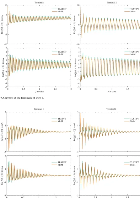
Figure 7.Currents at the terminals of wire 1.

-3 -1 1 3

Re

{ ¯ I2

(

l

=

0

)}

in

m

A

Terminal 1

TLST/PT MoM

-3 -1 1 3

Im

{ ¯ I2

(

l

=

0

)}

in

m

A

0 0.5 1 1.5 2

fin GHz

TLST/PT MoM

-3 -1 1 3

Re

{ ¯ I2

(

l

=

1

)}

in

m

A

Terminal 2

TLST/PT MoM

-3 -1 1 3

Im

{ ¯ I2

(

l

=

1

)}

in

m

A

0 0.5 1 1.5 2

fin GHz

TLST/PT MoM

(10)

and 3 at pointP2. The terminals are located at pointP0and

P3. These points determine the geometry of the wire, where

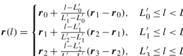
the position vector to a point Pν is denotedrν. In terms of the global parameterl, 0≤l≤1, the position vector to any point on the wire can be written as

r(l)=     

   

r0+

l−L0₀

L0₁−L0₀(r1−r0), L 0

0≤l < L

0

1

r1+

l−L0₁

L0₂−L0₁(r2−r1), L 0

1≤l < L

0

2

r2+

l−L0₂

L0₃−L0₂(r3−r2), L 0

3≤l≤L

0

2

(64)

withL0_i=Pi

k=1Lk/L, whereL00=0 and L

0

3=1. The

po-sition vector to a point on an arbitrarily shaped wire con-sisting ofnstraight segments can be expressed in the same way. The terminals at pointP0andP3are referred to as

ter-minal 1 and terter-minal 2, respectively. Figure 3 displays the computed currents at the terminals for a wire with segments of length L1=L3=0.5 m and L2=1.5 m, which implies

that segment 2 is parallel to the ground plane. The radius a for the thin wire approximation equals 0.25 mm. Simula-tions are performed in the frequency range from 1 MHz to 2 GHz, where the transmission line results are computed ap-plying the TLST/PT described in Sect. 3.2. The real and the imaginary parts of the currents at both terminals are in good agreement with method of moment (MoM) results over the entire frequency range which provides a first indication of the accuracy of the computed results. The number of resonances depends on the geometry of the wire and the frequency, since an integer multiple of half of the wavelength must approxi-mately be equal to the length of the wire. This leads to ap-proximately 34 resonances, in good agreement with the sim-ulated results forl=0 in Fig. 3.

Figure 4 displays the off-diagonal parameters P₁₂ and

P₂₁. The parameters are dependent on the position and are real-valued in the low frequency case. The graphs clearly show that the imaginary part vanishes along the entire length of the line. The parameters become complex-valued for higher frequencies, where the imaginary part comprises radi-ation losses. Results for the low frequency case which have been computed using the starting values of the TLST are shown in Fig. 5. The real and imaginary parts at both termi-nals agree well with the TLST/PT results up to a frequency of approximately 15 MHz.

As a second example, the currents in a two wire config-uration in the form of two semicircles is investigated. Ana-lytical solutions are known for a single circular loop (Nitsch and Tkachenko, 2005; Tkachenko and Nitsch, 2005; Storer, 1956; Wu, 1962), and for multiple loops (King and Harrison, 1969), where the solutions are expressed in terms of Fourier series. These solutions are limited to simple wire structures and cannot easily be extended to arbitrary wire configutions. The semicircles considered in this example are of ra-diusRand are separated by a distanced, as shown in Fig. 6. In order to apply the TLST/PT procedure, wire j is discre-tised withnjelements, where in this casejis equal to 1 or 2.

The terminals of wirej are located atPj,0andPj,nand are

referred to as terminal 1 and terminal 2 of wirej, respec-tively. The four terminals define a rectangle of width 2Rand heightd, and the two surfaces that are enclosed by the semi-circles and the ground plane are both perpendicular to the ground plane. Wire 1 is excited at terminal 1 with the same unit voltage source as in the first example. All remaining ter-minals are loaded with 50resistors. Simulations are per-formed with a semicircle radiusRof 1 m, a wire radiusa of 0.25 mm, a wire distanced of 0.5 m, and withn1=n2=60

segments. Figure 7 shows the currents at the terminals of wire 1 and Fig. 8 the currents at the terminals of wire 2. Good agreement of the TLST/PT and the method of moment results can be observed on all four terminals. This validates the procedure and confirms the applicability of the transmis-sion line procedure with perturbation approach to multi-wire problems.

5 Conclusions

A refined variant of the Transmission Line Super Theory that utilises perturbation theory, and which is referred to as TLST/PT, has been derived and applied to determine currents in thin wire structures. The perturbation approach enables a direct and non-iterative approximation of the initial cur-rent in a wire, which reduces the required computation time without compromising the accuracy of the results. The pro-cedure has been applied to compute the currents of a single wire problem and of a two wire configuration. TLST/PT and method of moment results have shown to be in good agree-ment, which validates the procedure and verifies applicability of the method to multi-wire problems.

Data availability. Data used in this article are available in the Sup-plement.

Supplement. The supplement related to this article is available online at: https://doi.org/10.5194/ars-16-123-2018-supplement.

Competing interests. The authors declare that they have no conflict of interest.

(11)

Acknowledgements. The authors would like to thank Jürgen Nitsch and Sergey Tkachenko for many valuable discussions on the topic. We acknowledge support by the Open Access Publication Funds of the SLUB/TU Dresden.

Edited by: Frank Gronwald

Reviewed by: Jürgen Nitsch and one anonymous referee

References

Bernstein, D.: Matrix Mathematics: Theory, Facts, and Formulas, 2nd Edn., Princeton reference. Princeton University Press, 2009. Burg, K., Haf, H., and Wille, F.: Band III Gewöhnliche Differential-gleichungen, Vol. 3 of Höhere Mathematik für Ingenieure, 4th Edn., B.G. Teubner Stuttgart, 2013.

Dollard, J. D. and Friedman, C. N.: Product Integration with Appli-cation to Differential Equations: Encyclopedia of Mathematics and its Applications, Cambridge University Press, Cambridge, 1984.

Gantmacher, F.: The Theory of Matrices, Number 2 in Chelsea Publishing Series, American Mathematical Society, Providence, 1960.

Haase, H.: Full-Wave Field Interactions of Nonuniform Transmis-sion Lines, PhD thesis, Otto-von-Guericke-Universität Magde-burg, 2005.

Heuser, H.: Gewöhnliche Differentialgleichungen, B.G. Teubner Stuttgart, 3rd Edn., 1995.

King, R. W. P. and Harrison, C. W.: Antennas And Waves: A Mod-ern Approach, The M.I.T. Press, Cambridge MA, 1969. Nitsch, J. and Tkachenko, S.: Global and modal parameters in the

generalized transmission-line theory and their physical meaning, Radio Science Bulletin, 312, 21–31, 2005.

Nitsch, J. and Tkachenko, S.: Propagation of Current Waves along Quasi-Periodical Thin-Wire Structures: Accounting of Radiation Losses, Interaction Notes 601, 2006.

Nitsch, J. and Tkachenko, S.: High-frequency multiconductor transmission-line theory, Found. Phys., 40, 1231–1252, 2010. Nitsch, J., Gronwald, F., and Wollenberg, G.: Radiating

Nonuni-form Transmission-Line Systems and the Partial Element Equiv-alent Circuit Method, Wiley, Chichester, West Sussex, 2009. Rambousky, R.: Analyse der Feldeigenschaften in offenen

TEM-Wellenleitern mit Methoden einer erweiterten Leitungstheorie, PhD thesis, Leibniz Universität Hannover, 2014.

Rambousky, R., Nitsch, J. B., and Garbe, H.: Application of the Transmission-Line Super Theory to Multiwire TEM-Waveguide Structures, IEEE T. Electromagn. C., 55, 1311–1319, 2013. Tesche, F. M., Ianoz, M. V., and Karlsson, T.: EMC Analysis

Meth-ods and Computational Models, Wiley, Chichester, West Sussex, 1997.

Tkachenko, S. and Nitsch, J.: On the electromagnetic field excitation of smoothly curved wires, in: IEEE 6th International Symposium on Electromagnetic Com-patibility and Electromagnetic Ecology, 115–121, https://doi.org/10.1109/EMCECO.2005.1513078, 2005. Steinmetz, T.: Ungleichförmige und zufällig geführte

Mehrfach-leitungen in komplexen technischen Systemen, PhD thesis, Otto-von-Guericke-Universität Magdeburg, 2006.

Storer, J. E.: Impedance of thin-wire loop antennas, Transactions of the American Institute of Electrical Engineers, Part I: Communi-cation and Electronics, 75, 606–619, 1956.