R E S E A R C H A R T I C L E
Open Access
A
Simulation App
based on reduced order
modeling for manufacturing optimization
of composite outlet guide vanes
Jose Vicente Aguado
1, Domenico Borzacchiello
1, Chady Ghnatios
2, François Lebel
3,
Ram Upadhyay
3, Christophe Binetruy
4and Francisco Chinesta
1**Correspondence:
[email protected] 1ICI-High Performance Computing Institute, Ecole Centrale Nantes, 1 rue de la Noe, 44300 Nantes, France Full list of author information is available at the end of the article
Abstract
Composites manufacturing processes usually involve multiscale models in both space and time, highly non-linear and anisotropic behaviors, strongly coupled multiphysics and complex geometries. In this framework, the use of simulation for real-time decision making directly in the manufacturing facility is still precluded nowadays, in spite of the impressive progresses reached in numerical analysis and computer science during the last decade. In this paper, a process-specific simulation tool based on reduced order modeling is introduced, theSimulation App. This concept is presented through a practical case involving a multi-physics and coupled problem describing the manufacturing process of a composite outlet guide vane. We show that several manufacturing settings can be simulated in few seconds with theSimulation App, thus enabling fast process optimization. Finally, the advantages over general-purpose simulation software, in the context of process simulation, are discussed.
Keywords: Simulation App, Reduced order modeling, Real time simulation, Numerical simulation, Composites forming processes, Curing, Consolidation, Proper Generalized Decomposition, Parametric solutions, Computational Vademecums
Background
Efficient simulation of composite manufacturing processes remains even nowadays, in many cases, a challenging issue, mainly when they involve rich 3D behavior, multi-physics and the necessity of solving many scenarios very fast for optimization purposes [1,2]. Com-posites manufacturing processes involve many different physics. For instance, impregna-tion of fibrous reinforcements involves flow models through porous media, combined with the mould compression for ensuring an appropriate degree of consolidation [3,4]. During consolidation the resin curing kinetics strongly affects its viscosity and therefore the flow conditions [5].
The intimate coupling between the resin flow, the reinforcement permeability, that decreases upon compression of the mould, and the viscosity, that depends on the tem-perature and the curing degree, can be at the origin of different process defects. Large viscosities imply high pressures that can generate irreversible preform deformations and
©The Author(s) 2017. This article is distributed under the terms of the Creative Commons Attribution 4.0 International License (http://creativecommons.org/licenses/by/4.0/), which permits unrestricted use, distribution, and reproduction in any medium, provided you give appropriate credit to the original author(s) and the source, provide a link to the Creative Commons license, and indicate if changes were made.
even local reinforcement displacements creating local inhomogeneity defects. Moreover, residual stresses are another manifestation of this intimate multi-physics coupling [1,6].
Another important issue encountered in the simulation of composites manufacturing is the one related to the process control and optimization [7–9]. In general, optimization implies the definition of a cost function and the search of the optimum process parameters defining the minimum of that cost function. The procedure starts by a guessed set of process parameters. Then the process is simulated using suitable numerical methods. The solution of the model is the most expensive step of the optimization procedure. As soon as the solution is available, the cost function can be evaluated and its optimality checked. If the chosen parameters do not define a minimum (at least local) of the cost function, the process parameters should be updated and the solution recomputed. The procedure continues until reaching the minimum of the cost function. The solution of the process model is a tricky task that demands important computational resources and usually implies extremely large computing times. Thus, usual optimization procedures are inapplicable under the real-time constraint. The same issues are encountered when dealing with inverse analysis in which material or process parameters are expected to be identified from numerical simulation, by looking for the unknown parameters so that computed fields match the ones measured experimentally.
Until now, the solution consisted in using the more and more powerful computing platforms and techniques for speeding up standard discretization techniques. Appealing alternatives for circumventing, or at least alleviating, these issues lie in the use of reduced order modeling (ROM) [10–12] strategies. ROM is based on the observation that the family of parametric solutions of a given model usually contains much less information than it was originally assumed when the discrete model was built. Proper Orthogonal Decomposition, Proper Generalized Decomposition and Reduced Basis are nowadays widely considered from a fundamental and applicative viewpoints.
Proper Orthogonal Decomposition (POD) is a general technique for extracting the most significant characteristics of a system’s behavior and representing them in a set of “POD basis vectors” [13,14]. These basis vectors then provide an efficient (typically low-dimensional) representation of the key system behavior, which proves useful in a variety of ways. The most common use is to project the system governing equations onto the reduced-order subspace defined by the POD basis vectors. This yields an explicit POD reduced model that can be solved in place of the original system. The POD basis can also provide a low-dimensional description in which to perform parametric interpolation [15,16], infill missing or “gappy” data [17], hyper-reduced approximations [18,19], and perform model adaptation. There is an extensive literature on POD showing it has broad application across fields. Some review of POD and its applications can be found in [20,21] and the references therein.
Techniques based on the use of separated representations are at the heart of the so-called Proper Generalized Decomposition (PGD) methods [28–30]. Such separated rep-resentations were considered in computational mechanics for separating space and time in transient solutions [31,32]. Separated representations were employed for solving mul-tidimensional models suffering the so-called curse of dimensionality [33–35] and in the context of stochastic modeling [36]. Then, they were extended for separating space coor-dinates making possible the solution of models defined in degenerated domains, e.g. plate and shells [37] as well as for addressing parametric models where model parameters were considered as model extra-coordinates, making possible the offline calculation of the para-metric solution that can be viewed as a metamodel or a computational vademecum, to be used online for real time simulation, optimization, inverse analysis and simulation-based control [38]. Some applications in the context of composites manufacturing processes were addressed in [39] while the multi physics coupling was successfully achieved in [40]. This work is intended to propose a first approach using reduced order modeling tech-niques to enhance adaptability of composite manufacturing process to changeable mate-rial and process environments through increased parametric modeling capabilities. The process selected is the consolidation and curing of a real part. Consolidation and curing of thermoset pre-impregnated fibers (from now on, simply referred as pre-pregs) involve different physics: heat transfer, compression of fiber beds, resin flow and chemical reac-tion. Strong couplings exist between these physics and many material parameters come into play. In this paper we combine several different modeling and simulation strategies for the efficient solution of a generic multi-physic and coupled problem. In particular, we propose a ROM-based segregated approach (rather than a monolithic one) for treating each physics separately. This approach allows applying, in each case, the most convenient ROM technique. Then, coupling is made by defining an appropriate parametrization of the coupling variables. A strategy for coupling ROMs of different kind (i.e. reduced solvers and parametric solutions) is also proposed. The integration of all these models constitutes a
Simulation Appthat allows real-time evaluation of any process conditions. The described methodology can be extended and generalized to other processing technologies.
Process description and physics modeling
The concept of aSimulation Appis presented in this paper through a practical application: the manufacturing process of a composite blade, and more specifically, an outlet guide vane. In this section we are first describing the manufacturing process from a technological point of view. Then we shall present the physics modeling and constitutive behavior for each considered physical phenomena.
Process description
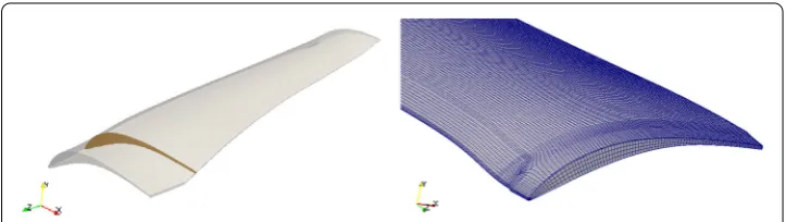
Figure1shows the geometry and the computational mesh of the composite OGV part, which is manufactured by press forming and curing of 66 thermoset unidirectional con-tinuous fiber pre-preg layers, i.e. fibers already impregnated with resin in a partially cured stage.
During the forming process, the composite lay-up is heated by conduction from the top and bottom metallic mold walls and consolidated under press. See Fig.2for details. The heat initiates the cure reaction and the applied pressure provides the force needed to drain the excess of resin out of the composite, to consolidate pre-preg layers and to reduce voids by compressing the air inside. The temperature raise determines the onset of the cure reaction. Because of the exothermic effects of the curing process and the variability of the kinetic and thermal properties of the resin with the temperature and curing degree, the process is highly nonlinear. Moreover, the resin undergoes a strong
Fig. 1 Global view of the OGV part geometry with cross sectional slice (left) and detail of the computational mesh (right)
rheological modification because its viscosity also depends on the temperature and the degree of cure. Therefore the flow conditions vary continuously with time.
The nominal heating cycle is designed so as to apply a constant temperature of 438 K (330 F) on both top and bottom mold walls. The press closure is initially based on a constant closure rate of 0.1524 mm/min (6 mils/min). As the cure reaction advances, the viscosity increases and so the closing force to be applied by the press increases. When the maximum closing force of the press is attained, the control switches to a force-based one. The closure rate is therefore adapted so as to keep the closing force constant. A final technological restriction to be taken into account is the so-calledhard-stop condition, occurring when the cumulated displacement reaches its maximum value, 3.3 mm (130 mils).
Remark 1 (On the simulation of the press control system) Observe that the manufacturing process simulation will be nonlinear due to the just described press control system. If a force-based control applies, one has to solve a nonlinear problem in order to find out the closure rate that keeps the force constant at its maximum value.
Thermo-kinetic model
The model governing thermo-kinetic is given by the following partial differential equa-tions:
ρCp(T,α)∂ T
∂t = ∇ ·λ∇T +ρHα˙ (1a)
˙
α=fkin(T,α), (1b)
whereT(x, t) andα(x, t) represent the temperature and curing degree fields, respectively. We shall refer to Eq. (1a) and to Eq. (1b) as the heat and kinetic equations, respectively. The curing function, denoted byfkin, is given by the phenomenological model by Kamal and Sourour [41], widely used to describe the conversion kinetics of epoxy systems:
fkin(T,α)=
k1exp
E1 RT
+k2αmexp
E2 RT
(1−α)n, (2)
Heat convection is neglected because of the creeping flow approximation and it is assumed there is no dispersion effect, i.e. resin and fiber share the same temperature. The coef-ficientsρandCpappearing in Eq. (1a) denote the density and the specific heat, whileλ stands for the thermal conductivity tensor of the composite part. These were obtained from the properties of the resin and fibers using a linear mixing rule. For the specific heat this reads:
Cp(T,α)=Vf Cpf +(1−Vf)Cpr, (3)
whereCpf andCprare the specific heat of the fibers (depending on the temperature) and the resin, respectively. At the initial conditions, i.e.Vf = Vf0=57%, it can be rewritten
as follows:
Cp(T,α)=(p1T+p0)α+(q1T+q0) (1−α), (4)
where coefficientsp0,p1,q0andq1are defined in Table1. Note that only this quantity
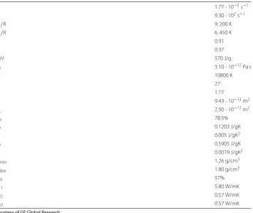
Table 1 Material parameters considered in the physical modeling of the OGV part manufacturing process
k1 1.77·10−5s−1
k2 9.30·102s−1
E1/R 9,200 K
E2/R 6,450 K
n 0.91
m 0.37
H 570 J/g
η0 3.10·10−12Pa s
B 10800 K
C 27
d 1.77
c 9.43·10−13m2
c⊥ 2.50·10−12m2
Vfa 78.5%
p0 0.1203 J/gK
p1 0.005 J/gK2
q0 0.5905 J/gK
q1 0.0019 J/gK2
ρresin 1.26 g/cm3
ρfiber 1.80 g/cm3
Vf0 57%
λ11 5.80 W/mK
λ22 0.57 W/mK
λ33 0.57 W/mK
Courtesy of GE Global Research
constants in the system considered in this application. The thermal properties, as well as the coefficients of the kinetic model, were obtained from experimental characterization and are summarized in Table1.
The solution of the thermo-kinetic model requires defining appropriate initial and boundary conditions. The initial conditions are given by T(x, t = 0) = T0 and α(x, t = 0) = α0. It is important to note that the heat equation, Eq. (1a), is global in
space whereas the kinetic equation, Eq. (1b) is local, that is, the solution at a particular location of the part only depends on the thermo-kinetic history at that location. Therefore, boundary conditions are only needed for the heat conduction equation, and in particular they concern the temperature cycle prescribed at the top and bottom surfacesS+ and S−, see Fig.3, that readT(x ∈ S+, t) = Tt(t) andT(x ∈ S−, t) = T
b(t), respectively. The heat losses through the lateral surfacesL(see Fig.3) can be neglected, that results in ∇T(x, t)·n=0, beingnthe unit outwards vector defined onL.
Consolidation model
During the consolidation under press, the excess of resin is drained out of the composite. Assuming that only the resin moves between fibers, that is, preform is compressed but remains nearly at rest, the resin flow model can be described from the Darcy’s flow model:
∇ ·v=0
Fig. 3 Boundary conditions description for the thermo-kinetic problem
wherev,Pandηare the velocity, pressure and viscosity fields andKis the permeability tensor. The solution of the flow model requires adequate boundary conditions. In par-ticular it is assumed that in the lateral boundaries L, see Fig.3, the pressure vanishes. On the other hand, it is assumed that the velocity at the top surface corresponds to the compression rate ˙Uimposed by the press, which is assumed to be directed vertically, while the resin velocity vanishes at the bottom surface. In summary:
⎧ ⎪ ⎨ ⎪ ⎩
P(x∈L)=0
v(x∈S+)=(0,0,−U˙)T
v(x∈S−)=0
. (6)
As the curing reaction advances, the resin viscosityηtends to increase until the flow is no longer possible or will induce fiber washing. This behavior is taken into account in the following chemo-rheological model:
η(T,α)=η0exp
B T
exp Cαd. (7)
The viscosity evolution is therefore the main link between Eqs. (1) and (5): the thermo-kinetic simulation influences the pressure field through the viscosity, which depends on both the temperature and the curing degree. Note also that, strictly speaking, the thermo-kinetic simulation depends on the consolidation simulation, because, as the excess of resin is drained out under the action of the press, the fiber volume fraction changes, and so the specific heat does, see Eq. (3). However, this link will be neglected in practice thanks to the semi-implicit linearization scheme that was implemented, see “Online simulation strategy: simulation modules coupling” section for details.
Finally, the permeability is also assumed to depend on the fiber volume fraction evolu-tion. The principal components obey the following expressions [42]:
K11=K22=c
(1−Vf)3
Vf2 and K33=c⊥
Vfa Vf −1
5/2
. (8)
Simulation based on reduced order modeling
In this section, we describe the simulation strategy, including the different simulation modules based on ROM techniques and their coupling. In particular, we recall the main features of the ROM methods that were implemented, emphasizing both the construction of the reduced models in the offline stage and their utilization in the online stage, as a part of theSimulation App.
The coupled model described in “Process description and physics modeling” section involves three primary unknown fields, the temperatureT(x, t), the pressureP(x, t) and the curing degreeα(x, t). The viscosity field,η(x, t), can be obtained as a post-processing of the temperature and curing degree fields. The nonlinearity associated to the coupling can be efficiently addressed by using a semi-implicit incremental time integration, and treating all coupling terms explicitly, therefore allowing for decoupling of the different problems. Thanks to this strategy, we are able to define different simulation modules, described below, one for each physics involved in the manufacturing process. This approach is particularly effective in the context of ROM, because it allows applying the most suitable techniques depending on the nature of the equations.
It is to be noted that domain changes due too the applied compression will be neglected, i.e. the mould thickness reduction remains small enough.
Reduced order modeling methods
The simulation strategy combines three different numerical techniques: (i) the Proper Orthogonal Decomposition (POD), (ii) the Discrete Empirical Interpolation Method (DEIM) and (iii) the Proper Generalized Decomposition (PGD). In this section we sum-marize the main ingredients of these three techniques.
The Proper Orthogonal Decomposition
POD extracts the most significant components, measured in 2-norm, in the solutions of a parametric problem from the analysis of a set of “snapshots” (previously computed solutions of a given problem at different times and for different values of the model parameters) and uses them to approximate the solution for a new set of parameters up to a certain degree of accuracy.
Thus, POD allows expressing the unknown field involved in a generic problemu(x, t;μ), withμthe vector containing the model parameters, as
u(x, t;μ)≈ Nu
n=1
anu(t;μ)φun(x), (9)
with usually much lowerNuthat the number of nodes, denoted byI, used for approximat-ing the unknown field within the finite element framework. When considerapproximat-ing discrete approximation spaces, the unknown vector at timetj,j=1,. . ., J, is denoted byu(tj;μ), that contains the value of the unknown field at each nodexi,i=1,. . ., I, can be expressed in the following reduced form:
u(tj;μ)=uau(tj;μ), (10)
The discrete empirical interpolation method
When considering a generic nonlinear functiong(u(x, t;μ)) its evaluation in the reduced state space from the coefficientsau(tj;μ) can be very expensive and, as discussed in [15,43], it may compromise the efficiency of reduced model techniques. One possibility consists of using the POD just described to extract a reduced basis able to approximate the nonlinear term as
g(x, t;μ)≈ Ng
n=1
ang(t;μ)φgn(x). (11)
In order to compute the approximation coefficientsang, withn=1,. . ., Ng, the nonlinear function is reconstructed at any timetjat onlyNgnodes, denoted byxgi, withi=1,. . ., Ng. The subscript•gstands for the fact of that points being related to the approximation of the nonlinear function on the reduced basis,φng. It results in the following linear system to be solved each at each time instance and given set of parameters:
⎛ ⎜ ⎜ ⎝
g(xg1, tj;μ) .. .
g(xgNg, tj;μ) ⎞ ⎟ ⎟ ⎠= ⎛ ⎜ ⎜ ⎝ φ1
g(x1g) · · · φ Ng
g (xg1) ..
. . .. ...
φ1
g(x Ng
g ) · · · φ Ng
g (x Ng g ) ⎞ ⎟ ⎟ ⎠ ⎛ ⎜ ⎜ ⎝
a1g(tj;μ) .. .
aNgg(tj;μ) ⎞ ⎟ ⎟
⎠. (12)
The remaining question concerns the choice of pointsxgi,i=1,. . ., Ng. These points are a priori arbitrary, the only contraint being that the matrix involved in Eq. (12) be invertible. However, in [43] authors propose to define these points using a greedy strategy in order to locate them to capture as much information as possible. The resulting points were called “magic points” and for the sake of completeness we describe below their calculation. We start by considering
x1
g =argmaxx|φg1(x)|. (13)
Then we computed1from
d1φg1(x1g)=φg2(x1g), (14)
that allows defining the residualr2(x), i.e. a contribution inφg2(x) that cannot be explained byφ1
g(x), from which computing pointxg2:
x2
g =argmaxx|r2(x)| with r2(x)=φ2g(x)−d1φg1(x). (15)
As by constructionr2(x1g)= 0 we can ensurexg2=xg1. The procedure is generalized for obtaining the other points involved in the interpolation procedure. Thus, for obtaining pointxgi we consider
xi
g=argmaxx|ri(x)| with ri(x)=φgi(x)− i−1
j=1
The coefficientsd1,. . ., di−1must be chosen for ensuring thatxgi =x j
g, ∀j< i. For this
purpose we enforce that the residual ri(x) vanishes at each locationxgj, withj < i by solving:
ri(xgj)=0=φgi(x j g)−
i−1
l=1 dlφgl(x
j
g), j=1,· · ·, i−1, (17)
that constitutes a linear system whose solution leads to the sought-after coefficients
d1,. . ., di−1.
The Proper Generalized Decomposition
Most of the existing model reduction techniques proceed by extracting a suitable reduced basis and then projecting the problem solution on it. Thus, the reduced basis construction precedes its use in the solution procedure, and one must be careful on the suitability of a particular reduced basis when employed for representing the solution of a particular problem.
This issue disappears if the approximation basis is constructed at the same time that the problem is solved. Thus, each problem has its associated basis in which its solution is expressed. One could consider few terms in its approximation, leading to a reduced representation, or all the terms needed for approximating the solution up to a certain accuracy level. The Proper Generalized Decomposition (PGD) proceeds in this manner.
When addressing the solution of a parametric problemu(x, t;μ) its PGD-based sepa-rated representation, including parameters as extra-coordinates, reads
u(x, t,μ)≈ Nu
n=1 φn
x(x)φtn(t)φμn(μ). (18)
For additional details the interested reader can refer to [38] and the numerous references therein.
The thermo-kinetic simulation module
A POD approach is applied in order to reduce the computational complexity of the thermo-kinetic simulation. Reduced basis are computed for both primary fields, tem-perature and curing degree. Other reduced basis are also computed in order to approx-imate nonlinearities using the DEIM. The training stage, i.e. snapshots generation, and the reduced basis extraction are explained in “Training stage and reduced basis extrac-tion” section. Then, in “Assembling the Reduced order model” section, the ROM for the thermo-kinetic simulation is assembled. The reduced version of the heat equation is formed by standard Galerkin projection onto the temperature reduced basis. The kinetic equation can be treated in a different manner thanks to its local nature. The computational complexity is reduced in this case by integrating Eq. (1b) only in a well-chosen subset of mesh nodes; in particular, that subset will be computed using DEIM.
Training stage and reduced basis extraction
• Initial degree of curing,α0, that may differ from one OGV part to another depending
on the time the pre-pregs stay out of the freezer before manufacturing.
• Initial temperature,T0, that may change depending on the ambient conditions.
• Temperature cycle imposed at both top and bottom walls of the mold, denoted by
Tt(t) andTb(t), respectively. In the actual process, however, a fixed temperature is kept all along the process, i.e. the variability at both the beginning and the end can be neglected. In addition, both top and bottom temperatures are the same in practice so we can simply denoteTc≡Tt =Tb.
• Initial fiber volume fraction,Vf0, that may change if the ply stack is modified by adding or removing plies.
We denote byμm = (α0, T0, Tc, Vf0)m, with 1≤ m ≤M, the parameter sampling in order to compute the snapshots. Recall that the objective is to train a ROM from these snapshots. The nonlinear thermo-kinetic coupled problem given by Eq. (1) was therefore solved to obtain the space-time temperature and curing degree space-time fields, i.e.
T(x, t;μm) andα(x, t;μm).
From these collected data, a reduced basis is extracted for both temperature and curing degree, allowing the introduction of the following approximations:
T(x, t;μ)≈ NT
n=1
anT(t;μ)φTn(x) and α(x, t;μ)≈ Nα
n=1
anα(t;μ)φαn(x), (19)
whereφnTandφnαdenote the temperature and curing degree basis functions, respectively. CoefficientsanTare to be determined by solving a reduced system, which will be formed by Galerkin projection onto the reduced basisφTn. On the other hand, coefficientsanαare to be determined by integrating the kinetic equation only in a subset of mesh nodes, denoted by{xnα}Nn=α1. This means that the kinetic equation may be integrated at onlyNαlocations (very few in practice) leading to important computational time savings. With the reduced basis for the curing degree at hand, these nodes are chosen straightforwardly as explained in “The Discrete Empirical Interpolation Method” section.
The nonlinear terms in the thermo-kinetic model, namely the specific heat and the curing function, also need a special treatment in order to build an efficient reduced solver. According to “The Discrete Empirical Interpolation Method” section, a reduced basis has to be formed for both specific heat and curing function.
Observe that the reduced basis for the curing degree can also be used to approximate the curing function. This is because the snapshots of the curing rate, ˙α(x, t;μm) (equivalently,
fkin(x, t;μm)), are linear combination of the snapshots of the curing degreeα(x, t;μm). Therefore, it is clear that the space spanned by both basis would be the same, and in consequence the curing function is approximated using the curing degree basis:
fkin(x, t;μ)≈ Nf
n=1
anf(t;μ)φfn(x) with φnf(x)≡φαn(x) (Nf =Nα). (20)
Regarding the specific heat approximation, the snapshotsCp(x, t;μm) are obtained sim-ply by evaluating Eq. (4) using the temperature and curing degree snapshots. Therefore, we introduce the following approximation:
Cp(x, t;μ)≈ NC
n=1
anC(t;μ)φCn(x), (21)
whereφn
Cdenote the specific heat basis functions. With the the reduced basis at hand, the corresponding DEIM points can be computed; we denote them by{xn
C} NC
n=1. Coefficients anCare to be determined by solving an interpolation problem, as explained in “The Discrete Empirical Interpolation Method” section.
Assembling the reduced order model
Let us first focus on the heat equation. We first introduce the approximations of the nonlinear terms, i.e. the specific heat and kinetic rate, given by Eqs. (20) and (21):
ρ ⎧ ⎨ ⎩ NC
n=1
anC(t;μ)φCn(x)
⎫ ⎬ ⎭∂
T ∂t =λ∇
2T +ρH
Nα
n=1
anf(t;μ)φnα(x)
. (22)
Remark 2 (On the approximation of the kinetic rate) As explained in “Training stage and reduced basis extraction” section, the kinetic rate is approximated using the basis for the curing degree, and so in the right-hand side of Eq. (22) we useφnα. However, it is worth to remark for the sake of clarity that we keep the coefficientsan
f, which are obviously not the same thanan
α.
Using a standard finite element discretization on the mesh, it results in the following discrete matrix form:
⎧ ⎨ ⎩
NC
n=1
anC(t;μ)Mn ⎫ ⎬
⎭T˙ +K T= Nα
n=1
anf(t;μ)bn
, (23)
whereMnare the different mass matrices, each one related to a specific heat basis function, φn
C(x);K is the conductivity matrix (not to be confused with the permeability tensor, although no distinct notation is used); andbnare the different source vectors related to each curing function basisφαn.
By performing the Galerkin projection of Eq. (23) onto the reduced basis for the temper-ature, denoted in its discrete form byT, and taking into account that discrete equivalent of Eq. (19) isT=TaT, we get:
⎧ ⎨ ⎩
NC
n=1
anC(t;μ) ˜Mn ⎫ ⎬
⎭a˙T +K a˜ T = Nα
n=1
anf(t;μ)˜bn
, (24)
with the following definitions for the reduced operators: ˜Mn = tTMnT ∈ RNT×NT, ˜
K=t
Finally, the reduced version of the kinetic equation is trivial thanks to its locality. In order to compute the coefficientsanαat each time, we are integrating Eq. (1b) at the DEIM points related to the curing degree:
˙
α(xnα, t;μ)=fkin(T(xαn, t;μ),α(xnα, t;μ)) with 1≤n≤Nα, (25)
which of course givesNαuncoupled ODEs. In discrete form:
˙˜
α(t;μ)=fkin( ˜T(t;μ),α˜(t;μ)), (26)
where ˙˜α,T˜,α˜ ∈ RNα×1. Coefficientsan
α(t;μ) in Eq. (19) are computed by solving the following interpolation problem:
α(xmα, t;μ)= Nα
n=1
anα(t;μ)φαn(xαm) with 1≤m≤Nα. (27)
Implementation details and results
We report hereafter the details for the numerical implementation of the full-order solver, used for computing the snapshots:
• The Finite Element mesh is composed of 116,136 HEX8 elements, with 147,245 nodes.
• A first-order semi-implicit integration scheme was applied. The simulated time is 2 h of process, with 20,000 time steps.
• A Preconditioned Conjugate Gradient is used as linear solver.
• The typical running time, for a single parameter execution, is 5 h on a 64bit machine with the following specifications: 2.9 GHz Intel Core i5 with 16 Gb 1867 MHz DDR3, running under MacOS X 10.10.5.
Concerning the snapshots generation, we considered random perturbations around the nominal parameters: μnominal = (α0 = 0, T0 = 288 K, Tc = 438 K, Vf0 = 57%).
The amplitude of the perturbations is in the following ranges: α0 ∈ [0,0.05] (+5%), T0∈[273,303] K (±5%),Tc∈[416,460] K (±5%),Vf0∈[50,64]% (±7%). Reduced basis
of the following dimension (i.e. number of degrees of freedom of the ROM) were found:
NT = 10,Nα = 7 andNC = 5, which proves the pertinency of using low dimensional approximations for the thermo-kinetic model. We report hereafter the details for the numerical implementation of the ROM solver:
• A variable order (1–5) Numerical Differentiation Formula (MATLAB ode15s) time integrator was used. The simulated time is 2 h and the number of time steps varies adaptively.
• The typical running time is in the range 1–10 seconds depending on the process conditions, using the same machine described previously. It is important to emphasize that the simulation took few seconds to completion instead of the many hours needed when solving the full order problem.
is 236 Mb. More details about the RAM consumption of the final implementation will be given in “ASimulation Appfor the OGV manufacturing process” section. • A posteriori validation of the reduced model was carried out by comparing results
with full-order FEM simulations for sets of randomly generated process parameters. The observed relative error measured in the maximum norm is typically of the order of 10−5.
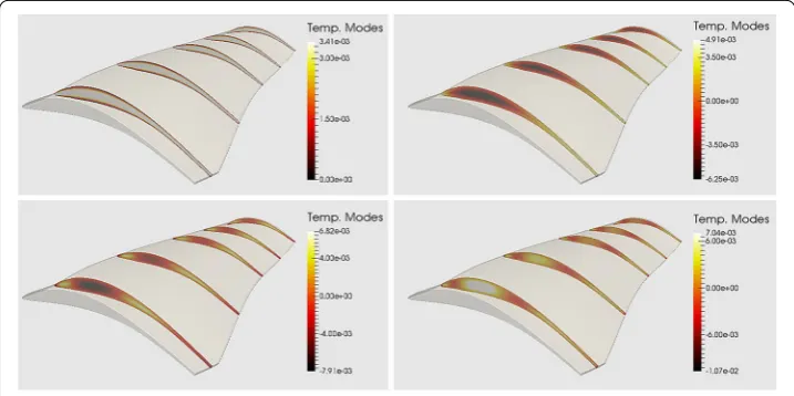
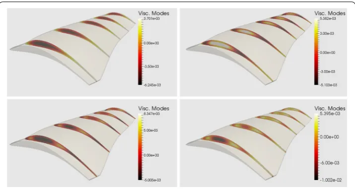
Figures4and5depict the first four modes (the most significant ones) of the temperature and the curing degree. Figure6shows the time evolution of the weights related to the temperature and degree of curing modes.
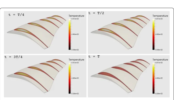
Figure 7represents the temperature solution issued from the reduced simulation, at four different times, after recombining the basis functions with the reduced coordinates.
Fig. 4 First four most significant temperature modes:φ1
T(x) (top-left);φT2(x) (top-right),φ3T(x) (bottom-left)
andφ4
T(x) (bottom-right)
Fig. 6 Time evolution of the temperature (left) and curing degree (right) reduced coordinates,an T(t;μ),
related to the first five temperature modes (i.e.n≤5) during the first 100 s of the simulation, corresponding to a randomly chosen parameter set
Fig. 7 Temperature fields at four different times from the thermo-kinetic ROM:t=T/4 (top-left);t=T/2 (top-right);t=3T/3 (bottom-left) andt=T(bottom-right)
The consolidation simulation module
The PGD method was applied in order to reduce the computational complexity of the consolidation model. Recall that the consolidation model is nonlinear itself, because the permeability tensor depends on the fiber volume fraction. However, as explained in “Con-solidation model” section, the permeability tensor can be assumed uniform, i.e. not varying through the domain. In consequence, observe that the problem could be linearized by sim-ply considering the permeability tensor as an extra-coordinate in the PGD framework. A similar approach was already addressed in the context of nonlinear soil dynamics [44]. Hence, in this scenario, we would have a parametric pressure field in the form:P(x,K). And more importantly, the computation of such parametric would now involve a linear problem. This can be understood by thinking of the parametric solution as being a linear solver inside a fixed-point nonlinear scheme.
approach to that one explained in “The thermo-kinetic simulation module” section. In fact, we are seeking for an approximation of the inverse of the viscosity field, see Eq. (5), as follows:
η−1(x, t;μ)≈
Nη
n=1
anη(t;μ)φnη(x), (28)
whereφn
ηdenotes the basis functions for the inverse of the viscosity, computed from snap-shotsη−1(x, t;μ
m), 1≤m≤M, by simple evaluation of Eq. (7). Observe that coefficients anηcan be seen in fact as the coordinates of the inverse of the viscosity on the reduced basis, at every instant and choice of parameters. We are therefore introducing them as extra-coordinates in the PGD parametric solution, i.e.P(x,K,aη). Such parametric solution is now able to provide the pressure field, not only for every possible permeability tensor, but also for every viscosity field living in the reduced basisφnη. Of course, we hopeNηto be small enough.
We shall explain in next section how to compute the coefficientsaηin order to be able to evaluate the parametric solution.
Remark 3 (On the dependence of the pressure field on the closure rate) Simulating the closure cycle of the press requires obtaining the pressure field, for a given viscosity field, permeability tensor (i.e. fiber volume fraction) and an imposed closure rate. However, it is worth to remark that the closure rate does not need to be considered as an extra-coordinate of the parametric solution, because of the linearity of the problem to be solved. In other words, the pressure field depends linearly on the closure rate.
The parametric solution of the flow problem, Eq. (29), within the PGD framework to obtain a separated representation of the parametric pressure field:
P(x,K,aη)= NP
n=1 φn
x(x)φKn(K)φan(aη). (29)
Even if such solution is related to a multidimensional problem, its linearity makes possible to compute it very efficiently by means of the PGD.
Implementation details and results
We report hereafter the details corresponding to the calculation of the PGD parametric pressure solution:
• The same mesh already described in “Implementation details and results” section was used.
• The inverse of the viscosity is parametrized usingNη=3 coordinates, corresponding to the first three modesφ1
η(x),φη2(x) andφη3(x) that can represent the 95% of the solution.
• The FE mesh for the viscosity in the phase-space (a1η, a2η, a3η) is made of 6,307 TET4 elements and 1387 nodes.
• The FE mesh for the permeability phase-spacek11, k22, k33is made of EDGE2 elements
1D×1D×1D, 100 nodes each.
Typical execution times are not reported for the consolidation ROM because they are completely negligible: evaluating the parametric pressure is straightforward.
Figure8depicts the first four modes (the most significant ones) of the inverse of the vis-cosity respectively, although only three were kept as explained before. The time evolution of the three associated coefficients,a1η(t),aη2(t) anda3η(t), describes a closed curve in the 3D espace defined by them, as depicted in Fig.9, since both the initial and final states are characterized by a uniform high viscosity field.
Finally Fig.10shows for four different rheologies expressed from vectoraηin the vis-cosity phase-space as well as their four associated pressure fields.
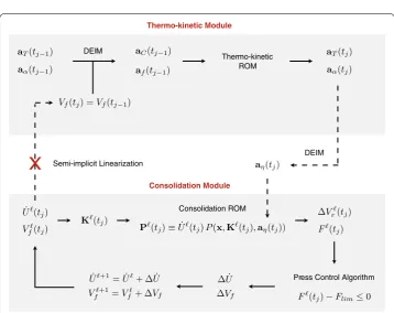
Online simulation strategy: simulation modules coupling
We summarize in this section the operation of the reduced models, with the help of Fig.11. Suppose that the reduced coordinates of the temperature and the curing degree are known from the previous time step; we denoteaT(tj−1) andaα(tj−1), respectively. Note
that at timet0, these reduced coordinates are obtained from the initial conditions for both
temperature and curing degree. Then:
Fig. 8 First four most significant inverse viscosity modes:φ1
η(x) (top-left);φ2η(x) (top-right),φη3(x) (bottom-left) andφ4
η(x) (bottom-right)
Fig. 9 Trajectory of coefficientsan
Fig. 10 Four examples showing arbitrary viscosities in the phase-space and their corresponding pressure field. For each example: (i) pressure field in the OGV part (left); (ii) reduced coordinates of the viscosity (red point) in the positive viscosities phase space (right)
DEIM
Thermo-kinetic ROM
Vf(tj) =Vf(tj−1)
Semi-implicit Linearization
aC(tj−1) af(tj−1) aα(tj−1)
aT(tj−1)
aα(tj) aT(tj)
aη(tj)
˙ U (tj) Vf(tj)
K(tj)
ΔVr(tj) F (tj)
Δ ˙U ΔVf ˙
U+1= ˙U + Δ ˙U V +1
f =Vf+ ΔVf
Press Control Algorithm
F (tj)−Flim≤0 P(tj)≡U˙ (tj)P(x,K(tj),aη(tj))
Consolidation ROM
DEIM
Thermo-kinetic Module
x
Consolidation Module
1. We evaluate both the specific heat and the curing function at the previous time step, i.e. a semi-implicit scheme is used. The reduced coordinates of both specific heat and curing function, denoted byaC(tj−1) andaf(tj−1) respectively, are computed using
DEIM.
2. With those reduced coordinates at hand, the thermo-kinetic ROM, Eqs. (24) and (26), can be assembled as explained in “The thermo-kinetic simulation module” section. 3. By performing a time increment, the reduced coordinates of both temperature and
curing degree can be obtained at timetj.
4. Then, the reduced coordinates of the viscosity,aη, can be computed by evaluating the chemo-rheology model and using DEIM.
5. With the previous information at hand, the consolidation module can be run. It involves solving a nonlinear problem because of the press control system, see “Process description” section. The nonlinear iterations are indexed by . We start by assuming that the closure rate is the same than in the previous time increment, i.e. ˙U =0(tj)=
˙
U(tj−1). Similarly, we considerVf=0(tj)=Vf(tj−1).
6. Using Eq. (8), the permeability tensor can be computed.
7. With the permeability tensor and the reduced coordinates of the viscosity, the para-metric PGD solution can be particularized. Recall that this solution has been com-puted for unitary velocity and so it must be scaled by the actual velocity. We denote byP (tj) the pressure field at timetjand iteration .
8. The velocity field can be then computed using Eq. (5). Integrating on the free bound-ary S, see Fig.3, the volume of resin drained can be computed,Vr. Note that knowing the loss of resin it is trivial to compute the current fiber volume fraction. 9. On the other hand, from the pressure field it is possible to obtain the vertical
com-ponent of the reaction force to be applied by the press so as to maintain the actual closure rate. The press force can be computed by integrating the pressure field on the upper boundaryS+, see Fig.3. However, note that this force only represents the fluid part, i.e. the resin, but it does not take into account the fiber contribution. In order to account for this extra contribution, we consider the Kim’s model.
10. With the press force,F (tj) at hand, the press control can be checked. A Newton-Raphson algorithm is used in order to compute both closure rate and fiber volume fraction correction, denoted byU˙ andVf.
11. From the corrections, both closure rate and fiber volume fraction can be updated. At convergence, we set: ˙U(tj)←U˙
∗
(tj) andVf(tj)←V
∗
f (tj), assuming the algorithm converges after ∗iterations.
12. Observe that the semi-implicit linearization allows excluding the thermo-kinetic module from the nonlinear problem. Otherwise, at each nonlinear iteration, it would be required to come back to the thermo-kinetic module, to recompute the specific heat, to solve the thermo-kinetic ROM, and so on.
ASimulation Appfor the OGV manufacturing process
order of half a second. However, since theSimulation Appis designed to be used directly in the manufacturing facility, the input and output delays are also relevant. As it will be explained later, both input and output interfaces were designed so as to enhance the user’s reactivity by restricting the input data to the bare minimum, while only relevant output information is displayed. Typically, a standard user takes no more than one minute in order to set up a new simulation, while the time consumed in visualizing and interpreting the results depends mostly on the user’s knowledge and experience.
The user interacts with the Simulation Appthrough a basic graphics user interface (GUI). In order to demonstrate the feasibility and potentiality of this kind of applications, we developed a demonstration version in the MATLAB® environment using GUIDE under MacOS X 10.10.5. This allows creating the GUI very easily. The MATLAB Application CompilerTMwas used in order to create a standalone executable file that could run outside MATLAB® and be easily transferred to the final user for demonstration purposes. The standalone version of theSimulation Apphas been tested on Microsoft Windows® 7 OS. Other proper implementations are of course possible although not explored in this paper, as they are outside of its scope.
The concept of aSimulation Appoffers several potentialities. Since the application is process-specific, rather than implementing a general purpose visualisation environment, it is possible to first identify the set of quantities of interest as output and then implement a simple and specific visualization interface. For example, if we know in advance that the maximum pressure gradient is an important indicator for defects, as it is the case in OGV manufacturing processes, we can include a functionality that displays the maximum pressure gradient and its location, at each time step. Then, the user can access to this information by simply activating a checkbox.
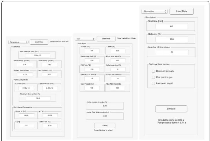
A similar discussion can be addressed regarding the data input. In a general purpose simulation software, a number of simulation parameters must be entered as user input. Although these have a significant impact within the modeling and simulation framework, they have little significance for the process designer. In order to get to these, the user must convert process parameters (physical measures, material properties) into simula-tion parameters (boundary and initial condisimula-tions, model adjustments) before running the simulation. TheSimulation App is designed to perform this conversion automatically according to rules provided beforehand. For instance, the initial fiber volume fraction is computed from process parameters, such as the following: area baseline plykit (stack of composite layers), the resin and fiber mass density, the mass of the convex and concave stack and the fiber areal weight (FAW) and the volatile content, see Fig.12. Therefore, the process designer only enters process parameters, which are the real meaningful infor-mation to them, without the need of expertise in multi-physics modeling or numerical methods. The difference between process and simulation parameters is kept transparent to the user in the GUI. By consequence, aSimulation Appis not only simulation tool but it also integrates the process knowledge via process-specific inputs and outputs.
TheSimulation Appis composed of three modules:
con-Fig. 12 Simulation Apppre-processing tabs: Parameters tab (left), Data Tab (center) and Simulation Tab (right)
version gathers data entered by the user and computes the simulation parameters. This operation is performed in the GUI via two different tabs: the Parameters Tab, in which some default values that normally do not change are proposed (e.g. resin and fiber specific weight), and the Data Tab, in which process parameters are defined (e.g. temperature cycle, closure rate, etc.) (see Fig.12). The conversion operation is launched by the Update button, and the initial degree of curing and the initial fiber volume content, both being simulation parameters, are computed.
2. SimulationThis module is driven by a principal function that governs the interaction between the two reduced models explained in previous sections: POD reduced model for the thermo-kinetic simulation and PGD reduced model for the consolidation simulation. Basically, this module takes all data defined in the pre-processing module and runs the ROM model in the time interval of interest defined by the user, as explained in “Online simulation strategy: simulation modules coupling” section. The user can also choose the number of equally spaced time frames at which the solution wants to be accessed. Additionally, the user can also demand to access to the solution at particular time frames of interest, such as minimum viscosity time frame, see Fig.12for details.
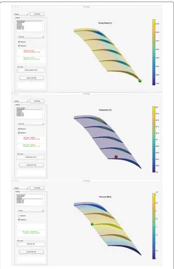
evolu-Fig. 13 Simulation Apppost-processing: Display tab. Curing degree field after 3.05 min (top). Temperature field at after 20.30 min (mid). Pressure field after 60 min (bottom)
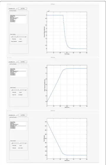
Fig. 14 Simulation Apppost-processing: quantities of Interest tab. Closure rate (top), fiber volume rate (mid) and part mass evolution (bottom) during the simulated time, 60 min
The RAM consumption of the MATLAB® implementation of theSimulation Appwas measured. Opening the application requires 239 Mb, whereas the amount of memory increases up to 504 Mb after loading data. The amount of memory required for running the simulation depends on the simulation timespan as well as on the process parameters. In the conditions already described in “Implementation details and results” section, 236 Mb are required on average, which brings the total to 740 Mb. However, the most demanding operation in terms of memory consumption is the Visualization module, which requires up to 1160 Mb. In general, the memory consumption could be drastically reduced in a proper (non demonstrator) implementation of the application. Some parts of the code could also be optimized, for instance, by avoiding reconstruction of the entire fields, since only some slices and the external surface are visualized.
ROM-basedSimulation Appscan be a powerful tool for complex composite processes to increase the entitlement yield by adapting for the variation that comes from material chemistry and physical properties in addition to thermal and pressure histories applied during the process. Typical entitlement yield is limited because of the inherent varia-tions and multi-physics interacvaria-tions. Part quality loss is due to either (i) internal defects, (ii) not meeting dimensional requirements or (iii) poor internal fiber matrix structure. A successful manufacturing process must minimize all three quality components. The
Simulation Appcan be implemented in the manufacturing process seamlessly to make real-time decisions regarding process adaptation possible overcoming inherent variation and truly increasing the entitlement yield of the process. As an example, theSimulation Appwill take real process measurements as inputs which capture the incoming variation in the pre-processing section and provide quantities of interest e.g. maximum pressure gradient that can be relate to quality. If the quality does not meet requirements, pre-computed sensitivity results can be used to identify corrective process change to bring it within requirements. The corrective process change can be as simple as choosing among predefined process cycles. All this can be made possible only because of real-time models capable of reflecting physics of the entire process.
Conclusions
In this paper we have introduced theSimulation Appconcept, a process-specific simula-tion tool based on reduced order modeling techniques. Using a combinasimula-tion of them, we were able to reduce from several hours to few seconds the computational time of a cou-pled multi-physics and strongly nonlinear model describing the manufacturing process of a composite outlet guide vane. Defining a coupling strategy between the different reduced order models was an essential part of this work. In particular, we presented an approach based on an appropriate parametrization of the coupling fields. The use of such fast simulation in a real-time decision making environment being possible, process-specific pre-processing and visualization functionalities were added, leading to theSimulation Appconcept.
to enter only process parameters while the simulation parameters are limited to the bare minimum. Similarly, the visualization module was designed so as to display only the relevant information, mainly the process indicators upon which decisions are made. Note that, by definition, process indicators are specific to a particular process, which is contrary to the spirit of general-purpose software. Therefore, theSimulation Appestablishes a link between process parameters and process indicators through a comprehensive numerical simulation which includes not only the physics and their couplings but also technological constraints such as the control loop of the process, if any.
Finally, even if the Simulation Apphas been presented on a case study of industrial interest, it is easy to imagine building similar tools for other manufacturing processes involving different physics, materials and technology.
Authors’ contributions
JVA and DB constructed the thermo-kinetic reduced order model and the Simulation App whereas CG constructed the parametric-PGD consolidation model. FL, RU and CB defined the problem, the thermo-mechanical model, performed material characterization and defined process and control parameters. Finally, FC coordinated and designed the global numerical simulation strategy in collaboration with JVA and DB. All authors read and approved the final manuscript.
Author details
1ICI-High Performance Computing Institute, Ecole Centrale Nantes, 1 rue de la Noe, 44300 Nantes, France,2Notre Dame University-Louaize, P.O. Box: 72, Zouk Mikael, Zouk Mosbeh, Lebanon,3Composite Technologies GE Global Research, One Research Circle, Niskayuna, NY 12309, USA,4GeM, Institute of Civil and Mechanical Engineering, Ecole Centrale Nantes, 1 rue de la Noe, 44300 Nantes, France.
Competing interests
The authors declare that they have no competing interests.
Received: 21 March 2016 Accepted: 4 January 2017
References
1. White SR, Hahn HT. Cure cycle optimization for the reduction of processing-induced residual stresses in composite materials. J Compos Mater. 1993;27(14):1352–78.
2. Pillai VK, Beris AN, Dhurjati P. Intelligent curing of thick section composites using a knowledge-based system. J Compos Mater. 1997;31(1):2251.
3. Shojaei A, Ghaffarian SR, Karimian SMH. Modeling and simulation approaches in the resin transfer molding process: a review. Polymer Compos. 2003;24(4):525–44.
4. Park CH, Woo L. Modeling void formation and unsaturated flow in liquid composite molding processes: a survey and review. J Reinf Plast Compos. 2011;30(11):957–77.
5. Kardos JL, Dudukovic MP, Dave R. Void growth and resin transport during processing of thermosettingmatrix com-posites. In: Epoxy resins and composites IV. Berlin: Springer, 1986. p. 101-23.
6. Zobeiry N, Vaziri R, Poursartip A. Computationally efficient pseudo-viscoelastic models for evaluation of residual stresses in thermoset polymer composites during cure. Compos Part A Appl Sci Manuf. 2010;41(2):247–56. 7. Mounier AL, Binetruy C, Krawczak P. Multipurpose carbon fiber sensor design for analysis and monitoring of the resin
transfer molding of polymer composites. Polymer Compos. 2005;26(5):717730.
8. Schmachtenberg E, zur Heide Schulte J, Topker J. Application of ultrasonics for the process control of resin transfer moulding (RTM). Polymer Test. 2005;24(3):330–8.
9. Lawrence JM, Hsiao KT, Don RC, Simacek P, Estrada G, Sozer EM, Stadtfeld HC, Advani SG. An approach to couple mold design and online control to manufacture complex composite parts by resin transfer molding. Compos Part A Appl Sci Manuf. 2002;33(7):981990.
10. Chinesta F, Keunings R, Leygue A. The proper generalized decomposition for advanced numerical simulations: a primer. Berlin: Springer; 2014.
11. Antoulas A, Sorensen D, Gugercin S. A survey of model reduction methods for large-scale systems. Contemp Math. 2001;280:193220.
12. Quarteroni A, Manzoni A, Negri F. Reduced basis methods for partial differential equations: an introduction. New York: Springer International Publishing; 2015.
13. Volkwein S. Model reduction using proper orthogonal decomposition. Lecture Notes. Graz: Institute of Mathematics and Scientific Computing, University of Graz; 2011.http://www.uni-graz.at/imawww/volkwein/POD
14. Willcox K, Peraire J. Balanced model reduction via the proper orthogonal decomposition. AIAA J. 2002;40(11):2323–30. 15. Chaturantabut S, Sorensen DC. Nonlinear model reduction via discrete empirical interpolation. SIAM J Sci Comput.
2010;32:2737–64.
16. Peherstorfer B, Butnaru D, Willcox K, Bungartz HJ. Localized discrete empirical interpolation method. SIAM J Sci Comput. 2014;36(1):A168–92.
18. Ryckelynck D, Vincent F, Cantournet S. Multidimensional a priori hyper-reduction of mechanical models involving internal variables. Comput Methods Appl Mech Eng. 2012;225:28–43.
19. Amsallem D, Zahr MJ, Choi Y, Farhat C. Design optimization using hyper-reduced-order models. Struct Multidiscip Optim. 2015;51(4):919–40.
20. Benner P, Gugercin S, Willcox K. A survey of projection-based model reduction methods for parametric dynamical systems. SIAM Rev. 2015;57(4):483–531.
21. Ryckelynck D, Chinesta F, Cueto E, Ammar A. On the a priori model reduction: overview and recent developments. Arch Comput Methods Eng State Art Rev. 2006;13(1):91–128.
22. Patera AT, Rozza G. Reduced basis approximation and a posteriori error estimation for parametrized partial differ-ential equations. Copyright MIT (2006–2015). MIT Pappalardo Monographs in Mechanical Engineering. 2007.http:// augustine.mit.edu.
23. Drohmann M, Haasdonk B, Ohlberger M. Reduced basis approximation for nonlinear parametrized evolution equa-tions based on empirical operator interpolation. SIAM J Sci Comput. 2012;34(2):A937–69.
24. Fritzen F, Leuschner M. Reduced basis hybrid computational homogenization based on a mixed incremental formu-lation. Comput Methods Appl Mech Eng. 2013;260:143–54.
25. Rozza G, Huynh DBP, Patera AT. Reduced basis approximation and a posteriori error estimation for affinely parametrized elliptic coercive partial differential equations. Archiv Comput Methods Eng. 2008;15(3):229–75. 26. Rozza G. Fundamentals of reduced basis method for problems governed by parametrized PDEs and applications. In:
Ladeveze P, Chinesta F, editors. CISM Lectures notes. Separated Representation and PGD based model reduction: fundamentals and applications. Vienna: Springer; 2014.
27. Hesthaven J, Rozza G, Stamm B. Certified reduced basis methods for parametrized partial differential equations. Berlin: Springer; 2015.
28. Ammar A, Mokdad B, Chinesta F, Keunings R. A new family of solvers for some classes of multidimensional par-tial differenpar-tial equations encountered in kinetic theory modeling of complex fluids. J Non Newton Fluid Mech. 2006;139:153–76.
29. Ammar A, Mokdad B, Chinesta F, Keunings R. A new family of solvers for some classes of multidimensional partial differential equations encountered in kinetic theory modeling of complex fluids. Part II: transient simulation using space-time separated representation. J Non Newton Fluid Mech. 2007;144:98–121.
30. Falco A, Nouy A. A Proper Generalized Decomposition for the solution of elliptic problems in abstract form by using a functional Eckart-Young approach. J Math Anal Appl. 2011;376:469480.
31. Ladevèze P. The large time increment method for the analyze of structures with nonlinear constitutive relation described by internal variables. Comptes Rendus Académie des Sciences Paris. 1989;309:1095–9.
32. Boucinha L, Gravouil A, Ammar A. Spacetime proper generalized decompositions for the resolution of transient elastodynamic models. Comput Methods Appl Mech Eng. 2014;255:67–88.
33. Chinesta F, Ammar A, Leygue A, Keunings R. An overview of the Proper Generalized Decomposition with applications in computational rheology. J Non Newton Fluid Mech. 2011;166:578–92.
34. Hackbusch W. Tensor spaces and numerical tensor calculus. 1st ed. Berlin-Heidelberg: Springer; 2012.
35. Lavedèze P, Chamoin L. On the verification of model reduction methods based on the Proper Generalized Decom-position. Comput Methods Appl Mech Eng. 2011;200(23–24):2032–47.
36. Nouy A. A generalized spectral decomposition technique to solve a class of linear stochastic partial differential equations. Comput Methods Appl Mech Eng. 2007;196:4521–37.
37. Bognet B, Leygue A, Chinesta F. Separated representations of 3D elastic solutions in shell geometries. Adv Modell Simul Eng Sci. 2014;1(1):1–4.
38. Chinesta F, Leygue A, Bordeu F, Aguado JV, Cueto E, Gonzalez D, Alfaro I, Ammar A, Huerta A. PGD based computational vademecum for efficient design, optimization and control. Arch Comput Methods Eng. 2013;20(1):31–59. 39. Chinesta F, Leygue A, Bognet B, Ghnatios Ch, Poulhaon F, Bordeu F, Barasinski A, Poitou A, Chatel S, Maison-Le-Poec S.
First steps towards an advanced simulation of composites manufacturing by automated tape placement. Int J Mater Form. 2014;7(1):81–92.
40. Borzacchiello D, Aguado JV, Chinesta F. Reduced order modelling for efficient process optimisation of a hot-wall chemical vapour deposition reactor. Int J Numer Methods Heat Fluid Flow. In press.
41. Kamal MR, Sourour S. Kinetics and thermal characterization of thermoset cure. Polymer Eng Sci. 1973;13(1):59–64. 42. Gebart B. Permeability of unidirectional reinforcements for RTM. J Compos Mater. 1992;26(8):1100–33.
43. Barrault M, Maday Y, Nguyen NC, Patera AT. An “empirical interpolation” method: application to efficient reduced-basis discretization of partial differential equations. Comptes Rendus Mathématique. 2004;339(9):667–72.