Volume 2008, Article ID 126859,8pages doi:10.1155/2008/126859
Research Article
Phasor Representation for Narrowband Active
Noise Control Systems
Fu-Kun Chen,1Ding-Horng Chen,1and Yue-Dar Jou1, 2
1Department of Computer Science and Information Engineering, Southern Taiwan University 1, Nan-Tai Street,
Yung-Kang City, Tainan County 71005, Taiwan
2Department of Electrical Engineering, ROC Military Academy, Feng-Shan City, Kaohsiung 83059, Taiwan
Correspondence should be addressed to Fu-Kun Chen,fkchen@ieee.org
Received 25 October 2007; Accepted 19 March 2008
Recommended by Sen Kuo
The phasor representation is introduced to identify the characteristic of the active noise control (ANC) systems. The conventional representation, transfer function, cannot explain the fact that the performance will be degraded at some frequency for the narrowband ANC systems. This paper uses the relationship of signal phasors to illustrate geometrically the operation and the behavior of two-tap adaptive filters. In addition, the best signal basis is therefore suggested to achieve a better performance from the viewpoint of phasor synthesis. Simulation results show that the well-selected signal basis not only achieves a better convergence performance but also speeds up the convergence for narrowband ANC systems.
Copyright © 2008 Fu-Kun Chen et al. This is an open access article distributed under the Creative Commons Attribution License, which permits unrestricted use, distribution, and reproduction in any medium, provided the original work is properly cited.
1. INTRODUCTION
The problems of acoustic noise have received much attention during the past several decades. Traditionally, acoustic noise control uses passive techniques such as enclosures, barriers, and silencers to attenuate the undesired noise
[1, 2]. These passive techniques are highly valued for
their high attenuation over a broad range of frequency. However, they are relatively large in volume, expensive at cost, and ineffective at low frequencies. It has been shown
that the active noise control (ANC) system [3–14] can
efficiently achieve a good performance for attenuating
low-frequency noise as compared to passive methods. Based on the principle of superposition, ANC system can cancel the primary (undesired) noise by generating an antinoise of equal amplitude and opposite phase.
The design concept of acoustic ANC system utilizing a microphone and of a loudspeaker to generate a canceling sound was first proposed by Leug [3]. Since the character-istics of noise source and environment are nonstationary, an ANC system should be designed adaptively to cope with these variations. A duct-type noise cancellation system based on adaptive filter theory was developed by Burgess [4] and
War-naka et al. [5]. The most commonly used adaptive approach
for ANC system is the transversal filter using the least mean
square (LMS) algorithm [6]. In addition, the feedforward
control architecture [6–8] is usually applied to ANC systems for practical implementations. In the feedforward system, a reference microphone, which is located upstream from the secondary source, detects the incident noise waves and supplies the controller with an input signal. Alternatively, a transducer is suggested to sense the frequency of primary
noise, if to place the reference microphone is difficult.
The controller sends a signal, which is in antiphase with the disturbance, to the secondary source (i.e., loudspeaker) for canceling the primary noise. In addition, an error microphone-located downstream picks up the residual and supplies the controller with an error signal. The controller must accommodate itself to the variation of environment.
The single-frequency adaptive notch filter, which uses
two adaptive weights and a 90◦ phase shift unit, was
developed by Widrow and Stearns [9] for interference
the normalized frequency is pointed. Generally, a periodic noise contains tones at the fundamental frequency and at several harmonic frequencies of the primary noise. This type of noise can be attenuated by a filter with multiple notches [12]. If the undesired primary noise containsM sinusoids,
then M two-weight adaptive filters can be connected in
parallel. This parallel configuration extended to multiple-frequency ANC has also been illustrated in [6]. In practical applications, this multiple narrowband ANC controller/filter
has been applied to electronic mufflers on automobiles in
which the primary noise components are harmonics of the basic firing rate. Furthermore, the convergence analysis of the parallel multiple-frequency ANC system has been proposed in [12]. It is found by Kuo et al. [12] that the convergence of this direct-form ANC system is dependent on the frequency separation between two adjacent sinusoids in the reference signal. In addition, the subband scheme and phase compensation have been combined with notch filter in the recent researches [13–15].
Using the representation of transfer function [6–13], the steady state of weight vector for the ANC systems can be determined and the convergence speed can be analyzed by eigenvalue spread. However, it can not explain the fact that the performance will be degraded at some frequencies. Based
on the concepts of phasor representation [16], this paper
discusses the selection of reference signals in narrowband
ANC systems to illustrate the effect of phase compensation
in delayed-X LMS approach [11]. The different selections
of signal phasor to the reference signal are considered to describe the operation of narrowband ANC systems. In addition, this paper intends to modify the structure of Kuo’s FIR-type ANC filter in order to achieve a better performance. This paper is organized as follows.Section 2briefly reviews the basic two-weight adaptive filter and the delayed two-tap adaptive filter in the single-frequency ANC systems. Besides, the solution of weight vectors will be solved by using the phasor concept. InSection 3, the signal basis is discussed and illustrated for the above-mentioned adaptive filters based on
the phasor concept. In Section 4, the eigenvalue spread is
discussed to compare the convergence speed for different
signal basis selections. The simulations will reflect the facts and discussions. Finally, the conclusions are addressed in
Section 5.
2. TWO-WEIGHT NOTCH FILTERING FOR ANC SYSTEM
The conventional structure of two-tap adaptive notch filter with a secondary-path estimate S(z) is shown in Figure 1
[6–8]. The reference input is a sine wave x(n) = x0(n) =
sin(ω0n), where f0 is the primary noise frequency and
ω0 =2π(f0/ fS) is the normalized frequency with respect to
sampling ratefS. For the conventional adaptive notch filter, a
90◦phase shifter or another cosine wave generator [17,18] is required to produce the quadrature reference signalx1(n)=
cos(ω0n). As illustrated inFigure 1,e(n) is the residual error
signal measured by the error microphone, andd(n) is the
primary noise to be reduced. The transfer function P(z)
represents the primary path from the reference microphone
to the error microphone, and S(z) is the secondary-path
Noise source
Sine wave generator
90◦ phase shift
P(z) d(n) + e (n)
x1(n) y(n−)
x0(n) S(z)
S(z)
S(z)
h0(n) h1(n)
y(n)
x1(n)
x0(n) LMS
Figure 1: Single-frequency ANC system using two-tap adaptive notch filter.
transfer function between the output of adaptive filter and the output of error microphone. The secondary signal y(n) is generated by filtering the reference signal x(n) =
[x0(n) x1(n)]T with the adaptive filter H(z) and can be
expressed as
y(n)=hT(n)x(n), (1)
where T denotes the transpose of a vector, and h(n) =
[h0(n)h1(n)]Tis the weight vector of the adaptive filterH(z).
By using the filtered-X LMS (FXLMS) algorithm [6–8], the reference signals,x0(n) andx1(n), are filtered by
secondary-path estimation filterS(z) expressed as
xi(n)=s(n)∗xi(n), i=0, 1, (2)
where s(n) is the impulse response of the
secondary-path estimate S(z), and∗denotes linear convolution. The adaptive filter minimizes the instantaneous squared error using the FXLMS algorithm as
h(n+ 1)=h(n) +μe(n)x(n), (3)
wherex(n)=[x0(n) x1(n)]T andμ >0 is the step size (or
convergence factor).
Let the primary signal bed(n) = Asin(ω0n+φP) with
amplitudeAand phaseϕP. And, assume that the phase and
amplitude responses of the secondary-pathS(z) at frequency ω0isφSandA, respectively. Since the filtering of
secondary-path estimate S(z) is linear, the frequencies of the output signal y(n) and the input signal y(n) will be the same. To perfectly cancel the primary noise, the antinoise from the output of the adaptive filter should be set asy(n)=sin(ω0n+
ϕP−ϕS).Therefore, the relationship y(n)=s(n)∗y(n)=
d(n) holds. In the following, the concept of phasor [16] is used for representing the system to solve the optimal weight solution instead of using the transfer function and control theory [6–8]. The output phasor of adaptive filter H(z) would be the linear combination of signal phasorsx0(n) and
x1(n), that is,
y(n)=sinω0n
h0(n) + cos
ω0n
h1(n)
=sinω0n+ϕP−ϕS
Noise source Sine wave generator
P(z) d(n)
+ e(n)
x(n)
z−D z−1
y(n−)
S(z)
h0(n) h1(n)
S(z)
y(n)
x(n)
LMS
Figure 2: Single-frequency ANC system using delayed two-tap adaptive filter.
Therefore, the optimal weight vector is readily obtained as
hNotch(ϕ)=
cos(ϕP−ϕS)
sin(ϕP−ϕS)
≡
cos(ϕ) sin(ϕ)
, (5)
which depends on the system parameterφ=φP−φS.
This conventional notch filtering technique requires two tables or a phase shift unit to concurrently generate the sine and cosine waveforms. This needs extra hardware or software resources for implementation. Moreover, the input signals, xi(n),i = 0, 1, should be separately processed in order to
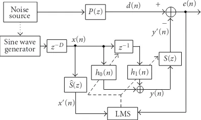
obtain a better performance. To simplify the structure, Kuo et al. [11] replaced the 90◦ phase shift unit and the two individual weights by a second-order FIR filter. As shown in
Figure 2, the structure does not need two quadratic reference
inputs and the filter-x process is reduced. Especially, Kuo et al. inserted a delay unit located in the front of the second-order FIR filter to improve the convergence performance for considering the implementation over the finite word-length machine. This inserted delay can be called the phase compensation to the system parameterφ=φP−φS. For Kuo’s
approach, the output phasor of adaptive filter would be the linear combination of sin(ω0(n−D)) and sin(ω0(n−D−1)),
whereDis the inserted delay. That is,
y(n)=sinω0(n−D)
h0(n) + sin
ω0(n−D−1)
h1(n)
=sinω0n+ϕ
.
(6)
Therefore, the optimal weight vector is the function ofD, ω0, andφshown as
hFIR
D,ω0,φ
= ⎡ ⎢ ⎢ ⎢ ⎣
sinω0(D+ 1) +φ
sin(ω0) −sinω0D+φ
sinω0
⎤ ⎥ ⎥ ⎥
⎦. (7)
To enhance the effect of delay-inserted approach, Kuo et
al. compared the performance with the case of no
phase-compensation (D=0) for the fixed-point implementation.
If no delay is inserted, that is, D = 0, the optimal weight
vector is simplified as
hFIR (D=0)
ω0,φ
= ⎡ ⎢ ⎢ ⎢ ⎢ ⎣
sinω0+φ
sin(ω0) −sin(φ) sinω0
⎤ ⎥ ⎥ ⎥ ⎥
⎦. (8)
Kuo et al. [11] have experimented and pointed out that the delay-inserted approach can improve the convergence per-formance for two-tap adaptive filter in some frequency band. Based on the phasor representation, the reference signals with different phase can further improve the performance of narrowband ANC systems.
3. SIGNAL BASIS SELECTION
In practical applications, adaptive notch filter is usually implemented on the fixed-point hardware. Therefore, the
finite precision effects play an important role on the
convergence performance and speed for the adaptive filter. It is difficult to maintain the accuracy of the small coefficient and to prevent the order of magnitude of weights from overflowing simultaneously, as the ratio of two weights in the steady state is very large. When the ratio of two weights in the steady state, limn→∞|h0(n)/h1(n)| = |h0/h1|, is close to one,
the dynamic range of weight value in adaptive processing
is fairly small [11]. Thus, the filter can be implemented
on the fixed-point hardware with shorter word length, or the coefficients will have higher precision (less coefficient quantization noise) for given a word length.
Based on the concepts of signal space and phasor, the relationship of signal phasors for the above-mentioned
two-weight adaptive filters is shown in Figure 3. Figure 3(a)
illustrates that the combination of the signal bases (phasors), sin(ω0n) and cos(ω0n), with the respective components in
h =[h0
h1], is able to synthesize the signal phasor y(n). Since the weight vectorh=hNotch(φ) is only the function of system
parameterφ, it is difficult to control the ratio of these two weights in steady state by the designer.Figure 4shows that only some narrow regions in the (φ,ω0)-plane with specified
values of φ satisfy the condition 1−ε < |h0/h1| < 1 +ε
(i.e., 1−ε < |cos(φ)/sin(φ)| < 1 +ε), where εis a small value. If the FIR-type adaptive filter [11] is used,Figure 3(b)
shows the relationship of the signal phasors y(n), sin(ω0n)
and sin(ω0(n−1)), where the inserted delayD = 0 holds.
Figure 5illustrates that the desired regions, in which the ratio
of two taps satisfies 1−ε <|sin(ω0+φ)/sin(φ)|<1 +ε(ε=
0.1), in (ω0,φ)-plane have been rearranged. We can find that
there are two solutions to achieve the requirement, 1−ε <
|h0/h1| < 1 +ε. One solution is to translate the operation
point along the vertical axis (ω0-axis) by way of changing the
sampling frequency. Therefore, the ratio of two weights for the optimal solution hFIR (D=0)(ω0,φ) can be controlled by
changing the sampling frequency to design the normalized
frequency ω0. That is, when the system parameter φ and
the primary noise frequency f0 are given, the designer can
adjust the sampling rate fS to locate the operation point S
h0·sin(ω0n)
h1·cos(ω0n)
y(n)
(a)
h1·sin(ω0(n−1))
h0·sin(ω0n)
y(n) sin(ω0n)
(b)
h0·sin(ω0(n−D))
h1·sin(ω0(n−D−1))
y(n)
(c)
h0·sin(ω0(n−Δ1))
h1·sin(ω0(n−Δ2))
y(n)
(d)
Figure3: Relationship of signal phasors for different two-taps filter structures. (a) Orthogonal phasors. (b) Single-delayed phasors. (c) Single-delayed phasors with phase compensation. (d) Near orthogonal phasors.
Normalized phaseφ(π)
−1 −0.5 0 0.5 1
N
o
rmaliz
ed
fr
eq
ue
ncy
ω0
(
π
)
0 0.1 0.2 0.3 0.4 0.5 0.6 0.7 0.8 0.9 1
Figure 4: The desired regions in (ω0,φ)-plane for conventional two-weight notch filter (ε=0.1).
is that we can shift the operation point along the horizontal axis to locate the operation point S in the desired region by
compensating the system phaseφ.
If the multiple narrowband ANC systems are used, the same sampling frequency is suggested such that the synthesis noises for secondary source can therefore work concurrently. If the sampling rate has been fixed, Kuo et al. [11] suggested inserting a delay unit to control the quantity of weights. The inserted delay can compensate the system phase parameter
φ = φP −φS. This system-phase compensation can move
the operation point from Sto Wi (i = 1,. . ., 4) along the
φ-axis, as shown inFigure 5. When the system phase has
been compensated, the operation point in (ω0,φ)-plane can
locate in the desired region which the ratio of two weights
is close to one. Using the signal bases sin(ω0(n−D)) and
sin(ω0(n−D−1)), the ratio of two weights satisfies
h0
h1 =sin
ω0(D+ 1) +φ
sinω0D+φ
=1. (9)
The solution to (9) isω0D= −φ−ω0/2±kπ/2, wherekis
any integer. The optimal delayDcan be expressed as D =
[(−φ/2π±k/4)(fS/ f0)−1/2] samples, where the operation
[·] denotes to take the nearest integer. These solutions
confirm the results in [11] in which the solution is derived by transfer-function representation. Besides, since the rela-tionship−π < ω0D < πholds, there are four solutions for
delayD; these solutions are the possible operation points, W1,W2,W3, andW4, as shown inFigure 5. From the phasor
point of view, the operation pointsW1andW3mean that the
synthesis phasory (n) is located in the acute angle formed by basis phasors sin(ω0(n−D)) and sin(ω0(n−D−1)), as
shown inFigure 3(c). Therefore, the range of weights value can be efficiently used. In addition, observingFigure 5, it can be found that the area of the desired regions varies with the normalized frequencies. It means that the performance will vary with the normalized frequency. This fact also confirms the experimental results in [11]. To solve the problem that the performance depends on the normalized frequency, another signal bases should be found for the two-tap adaptive filters. In the desired signal space, the phasors sin(ω0(n−D))
and sin(ω0(n−D−1)) are linearly independent but not
orthogonal. Based on the convergence comparison [19]
according to the eigenvector and eigenvalue, the convergence speed of Kuo’s FIR-type approach will be slow. To accelerate the convergence speed, the signal bases can be setup as
orthogonal as possible. As shown in Figure 3(d), the near
orthogonal bases sin(ω0(n − Δ1)) and sin(ω0(n − Δ2))
should be found to improve the performance. Based on this motivation, a new delay unit z−(Δ2−Δ1), (Δ
2−Δ1) ≥ 1 is
Normalized phaseφ(π)
−1 −0.5 0 0.5 1
N o rmaliz ed fr eq ue ncy ω0 ( π ) 0 0.1 0.2 0.3 0.4 0.5 0.6 0.7 0.8 0.9 1
W1 W2S W3 W4
Figure5: The desired regions in (ω0,φ)-plane for the delayed two-taps adaptive filter (ε=0.1).
Noise source Sine wave generator
P(z) d(n)
+ e(n)
z−Δ1 z−(Δ2−Δ1)
y(n) −
S(z)
h0(n) h1(n)
S(z)
y(n)
x(n)
LMS
Figure6: Single-frequency ANC system using proposed two-tap adaptive filtering.
of the proposed two-tap adaptive filter is therefore obtained as
hFIR,opt
Δ1,Δ2,ω0,φ = ⎡ ⎢ ⎢ ⎢ ⎢ ⎣
sinω0Δ2+φ
sinω0
Δ2−Δ1
−sinω0Δ1+φ
sinω0
Δ2−Δ1 ⎤ ⎥ ⎥ ⎥ ⎥
⎦, (10)
such that the signal y(n) can be represented as a linear
combination of sin(ω0(n−Δ1)) and sin(ω0(n−Δ2)). That
is,
y(n)=sin(ω0(n−Δ1))h0(n) + sin(ω0(n−Δ2))h1(n) =sin(ω0n+ϕ).
(11)
Since the signal bases in the proposed two-tap adaptive filter can be controlled by the delaysΔ1 andΔ2, the signal bases
can be setup as orthogonal as possible in order to accelerate the convergence speed and to compensate the system phase. Therefore, the delay (Δ2−Δ1) = max{[fS/4f0], 1}should
hold such that the signal phasor sin(ω0(n−Δ2)) can be
approximated as close as possible to cos(ω0(n−Δ1)). The
ratio of two weights will be close to one when the system phase has been compensated by the delayΔ1. That is,
h0
h1 =sin
ω0Δ2+φ
sinω0Δ1+φ
=sin
ω0
Δ1+fS/4f0
+φ sinω0Δ1+φ
≈1.
(12)
The solution to (12) isω0Δ1 = −φ−ω0(fS/8f0)±kπ/2,
k ∈ Z. The optimal delays can therefore be found as
Δ1 = [(−φ/2π −1/8±k/4)(fS/ f0)] samples. The desired
regions in (ω0,φ)-plane for the proposed two-tap adaptive
filter are similar to that of the desired regions shown in
Figure 4. Theoretically, the desired regions do not depend
on the normalized frequency in theory. To achieve a better performance for fixed-point implementation, the operation point in (ω0,φ)-plane can be shifted to the desired area along
the horizontal axis (φ-axis) after the delayΔ1is inserted.
4. DISCUSSION AND SIMULATIONS
The data covariance matrix for the conventional two-weight notch filter is described as [9]
RNotch=E
x(n)xT(n)= 1
2 1 0 0 1 . (13)
It is evident that both the corresponding eigenvalues are equal to 1/2. This leads to the fact that eigenvalue spread is one; the conventional two-weight notch filter has the better performance on However, since the optimal weight
hNotch(φ)=
cos(φ) sin(φ)
(14)
depends on the system phase parameterφ, the convergence
performance will depend on φ. For the Kuo’s FIR-type
adaptive filter [11], the data covariance matrix is
RFIR=
1 2
⎡
⎣ 1 cos(ω0)
cos(ω0) 1
⎤
⎦. (15)
The corresponding two eigenvalues are (1/2)[1±cosω0]; the
eigenvalue spread is
ρFIR= λmax
λmin =
1 +cosω0
1−cosω0 >
1. (16)
Since the eigenvalue spread ρFIR is larger than one, the
convergence speed will be slower than the conventional two-weight notch filter. It can be found that the convergence speed will depend on the normalized frequencyω0.
The proposed two-tap adaptive filter uses the data co-variance:
RFIR,opt=
1 2
⎡
⎣ 1 cos
ω0
Δ2−Δ1
cosω0
Δ2−Δ1
1
⎤ ⎦.
The corresponding eigenvalue spread is
ρFIR,opt=λmax
λmin =
1 +cosω0
Δ2−Δ1
1−cosω0
Δ2−Δ1.
(18)
Using the optimal delay found in (12), the data covariance is
RFIR,opt=1
2
⎡ ⎢ ⎢ ⎢ ⎣
1 cos
ω0 f
S
8f0
cos
ω0
fS
8f0
1
⎤ ⎥ ⎥ ⎥
⎦, (19)
and the corresponding eigenvalue spread isρFIR,opt = 1 +
|cos(ω0[fS/8f0])|/1 − |cos(ω0[fS/8f0])| ≈ 1. Since the
eigenvalue spread has been reduced from 1 +|cosω0|/1− |cosω0|to≈1, the proposed two-tap adaptive filter will have
higher convergence speed.
In the following simulations, the primary noise is set as d(n)=cos(ω0n+ϕP) +r(n), whereϕPis a random phase and
r(n) is the environmental noise with powerσ2
n. The primary
noise with frequency f0Hz is sampled with a fixed rate fS=
1000 Hz. The ratio of the primary noise to environmental noise for the signal is defined as SNR=10 log(1/2σ2
n) (dB).
All the examples are simulated with SNR = 20 dB. The
phase response of the secondary-path has been experimented to obtain a determined delay according to the designed sampling rate and frequency of primary noise. In addition, all input data and filter coefficients are quantized using word length of 16 bits within fraction length, and 8 bits to simulate the operation of fixed-point hardware. The temporary data is represented by 64-bit precision, and the rounding is performed only after summation. Therefore, the step size in FXLMS algorithm isμ=2×10⁻⁸, which is the precision of this simulation. All the learning curves are obtained after 200
independent runs with random system parameters φP. For
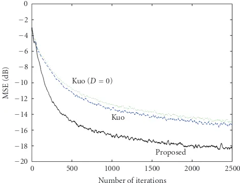
the frequency of primary noise f0 = (ω0/2π)fS = 100 Hz,
Figure 7illustrates that Kuo’s delayed two-tap adaptive filter
can improve the performance of the nondelayed one, but the convergence speed is still slow. Besides, the proposed approach, which is with well-selected bases, has the fast convergence speed and the best convergence performance.
In theory, the convergence performance of the proposed approach does not depend on the normalized frequency. However, simulations could not verify this statement and it also could not be explained by the representation of transfer function. Based on the concept of phasor rotation, we can find that the location of possible synthesis phasors would have variation for each adaptation if the number of samples in a cycle is not an integer, for example, fS/ f0 =
1000/97. The phasor-location variation will be significant as the amplitude of synthesis phasors increasing and will also lead to degradation in performance.Figure 8illustrates that Kuo’s approach and the proposed approaches are degraded in performance when the frequency of primary noise is 97 Hz with the sampling rate 1000 Hz. In addition,
when the normalized frequency is low, for example, f0 =
50 Hz, the angle of signal-basis phasors is small. In this case, the phase compensation is more important for Kuo’s FIR-type adaptive filter. Figure 9illustrates that the phase compensation can greatly improve the performance for the
Number of iterations
0 500 1000 1500 2000 2500
MSE
(dB)
−20 −18 −16 −14 −12 −10 −8 −6 −4 −2 0
Kuo (D=0)
Kuo
Proposed
Figure 7: Comparison of convergence performance for fS/ f0 = 1000/100.
Number of iterations
0 500 1000 1500 2000 2500
MSE
(dB)
−20 −18 −16 −14 −12 −10 −8 −6 −4 −2 0
Kuo (f0=97)
Kuo (f0=100)
Proposed (f0=100) Proposed (f0=97)
Figure 8: Comparison of convergence performance for different frequencies.
Number of iterations
0 500 1000 1500 2000 2500
MSE
(dB)
−20 −18 −16 −14 −12 −10 −8 −6 −4 −2 0
Kuo (D=0)
Kuo
Proposed
Number of iterations
0 500 1000 1500 2000 2500
MSE
(dB)
−20 −18 −16 −14 −12 −10 −8 −6 −4 −2 0
Kuo (D=0) Kuo Proposed
Figure10: Comparison of convergence performance for fS/ f0 = 1000/240.
case of low frequency for Kuo’s FIR-type adaptive filter. However, the convergence speed of Kuo’s two-tap adaptive filter is extremely low, since their eigenvalue spread is large; in this simulation, the eigenvalue spread is 39.8635. In addition, when the normalized frequency is close to 0.5, the eigenvalue spread of all approaches is close to 1 and the angle of the signal bases is inherently near-orthogonal. Therefore, the convergence speed for all approaches will be the same. For example, when the frequency of the primary noise is set as
f0 =240 Hz, all the approaches have the same convergence
performance and speed as illustrated inFigure 10. Observing
Figure 10, the performance of the phase-compensated and
noncompensated approaches is the same, since the 16-bit fixed-point hardware with 8-bit fraction length is enough for this simulation. These experiments confirm the results
presented in [11], in which their experiments found that
there is no improvement for convergence performance when the normalized frequency is 0.5. Observing Figures7–10, the proposed approach not only achieves a good performance, but also preserves the FIR adaptive filter structure.
5. CONCLUSION
In this paper, the phasor representation instead of transfer function is introduced and discussed for the narrowband ANC systems. Based on the concepts of signal basis and phasor rotation, the reference signal/phasor for two-tap adaptive filters has been modeled and well-selected. Using the representation of phasor can explain the reason why the performance of the narrowband ANC systems is degraded for some normalized frequency. In addition, to achieve a better performance, the proposed two-tap adaptive filter can choose the near-orthogonal phasors for the fixed-point hardware implementation. With the same complexity, the inserted delay in Kuo’s two-tap adaptive filter can be moved
back to construct the proposed approach, which would achieve a better performance.
REFERENCES
[1] C. M. Harris,Handbook of Acoustical Measurements and Noise Control, McGraw-Hill, New York, NY, USA, 3rd edition, 1991. [2] L. L. Beranek and I. L. Ver, Noise and Vibration Control Engineering: Principles and Applications, John Wiley & Sons, New York, NY, USA, 1992.
[3] P. Leug, “Process of silencing sound oscillations,” US patent no. 2043413, 1936.
[4] J. C. Burgess, “Active adaptive sound control in a duct: a computer simulation,”The Journal of the Acoustical Society of America, vol. 70, no. 3, pp. 715–726, 1981.
[5] G. E. Warnaka, J. Tichy, and L. A. Poole, “Improvements in adaptive active attenuators,” inProceedings of Inter-Noise, pp. 307–310, Amsterdam, The Netherlands, October 1981. [6] S. M. Kuo and D. R. Morgan,Active Noise Control Systems:
Algorithms and DSP Implementations, John Wiley & Sons, New York, NY, USA, 1996.
[7] S. M. Kuo and D. R. Morgan, “Active noise control: a tutorial review,”Proceedings of the IEEE, vol. 87, no. 6, pp. 943–973, 1999.
[8] P. A. Nelson and S. J. Elliott,Active Control of Sound, Academic Press, San Diego, Calif, USA, 1992.
[9] B. Widrow and S. D. Stearns, Adaptive Signal Processing, Prentice-Hall, Englewood Cliffs, NJ, USA, 1985.
[10] E. Ziegler Jr., “Selective active cancellation system for repeti-tive phenomena,” US patent no. 4878188, 1989.
[11] S. M. Kuo, S. Zhu, and M. Wang, “Development of optimum adaptive notch filter for fixed-point implementation in active noise control,” inProceedings of the International Conference on Industrial Electronics, Control, Instrumentation, and Automa-tion, vol. 3, pp. 1376–1378, San Diego, Calif, USA, November 1992.
[12] S. M. Kuo, A. Puvvala, and W. S. Gan, “Convergence analysis of narrowband active noise control,” inProceedings of the International Conference on Acoustics, Speech and Signal Processing (ICASSP ’06), vol. 5, pp. 293–296, Toulouse, France, May 2006.
[13] Y. Kinugasa, J. Okello, Y. Itoh, M. Kobayashi, and Y. Fukui, “A new algorithm for adaptive notch filter with sub-band filtering,” inProceedings of the IEEE International Symposium on Circuits and Systems (ISCAS ’01), vol. 2, pp. 817–820, Sydney, Australia, 2001.
[14] V. DeBrunner, L. DeBrunner, and L. Wang, “Sub-band adaptive filtering with delay compensation for active control,” IEEE Transaction on Signal Processing, vol. 52, no. 10, pp. 2932–2937, 2004.
[15] L. Wang, M. N. S. Swamy, and M. O. Ahmad, “An efficient implementation of the delay compensation for sub-band filtered-x least-mean-square algorithm,”IEEE Transactions on Circuits and Systems II, vol. 53, no. 8, pp. 748–752, 2006. [16] J. H. McClellan, R. W. Schafer, and M. A. Yoder, Signal
Processing First, Prentice-Hall, Upper Saddle River, NJ, USA, 2003.
[18] S. M. Kuo and W. S. Gan,Digital Signal Processors: Architecture, Implementations and Applications, Prentice-Hall, Englewood Cliffs, NJ, USA, 2005.