Volume 2007, Article ID 51563,14pages doi:10.1155/2007/51563
Research Article
Perceptual Coding of Audio Signals Using Adaptive
Time-Frequency Transform
Karthikeyan Umapathy and Sridhar Krishnan
Department of Electrical and Computer Engineering, Ryerson University, 350 Victoria Street, Toronto, ON, Canada M5B 2K3
Received 22 January 2006; Revised 10 November 2006; Accepted 5 July 2007
Recommended by Douglas S. Brungart
Wide band digital audio signals have a very high data-rate associated with them due to their complex nature and demand for high-quality reproduction. Although recent technological advancements have significantly reduced the cost of bandwidth and minia-turized storage facilities, the rapid increase in the volume of digital audio content constantly compels the need for better compres-sion algorithms. Over the years various perceptually lossless comprescompres-sion techniques have been introduced, and transform-based compression techniques have made a significant impact in recent years. In this paper, we propose one such transform-based com-pression technique, where the joint time-frequency (TF) properties of the nonstationary nature of the audio signals were exploited in creating a compact energy representation of the signal in fewer coefficients. The decomposition coefficients were processed and perceptually filtered to retain only the relevant coefficients. Perceptual filtering (psychoacoustics) was applied in a novel way by analyzing and performing TF specific psychoacoustics experiments. An added advantage of the proposed technique is that, due to its signal adaptive nature, it does not need predetermined segmentation of audio signals for processing. Eight stereo audio sig-nal samples of different varieties were used in the study. Subjective (mean opinion score—MOS) listening tests were performed and the subjective difference grades (SDG) were used to compare the performance of the proposed coder with MP3, AAC, and HE-AAC encoders. Compression ratios in the range of 8 to 40 were achieved by the proposed technique with subjective difference grades (SDG) ranging from –0.53 to –2.27.
Copyright © 2007 K. Umapathy and S. Krishnan. This is an open access article distributed under the Creative Commons Attribution License, which permits unrestricted use, distribution, and reproduction in any medium, provided the original work is properly cited.
1. INTRODUCTION
The proposed audio coding technique falls under the trans-form coder category. The usual methodology of a transtrans-form- transform-based coding technique involves the following steps: (i) transforming the audio signal into frequency domain coef-ficients, (ii) processing the coefficients using psychoacous-tic models and computing the audio masking thresholds, (iii) controlling the quantizer resolution using the masking thresholds, (iv) applying intelligent bit allocation schemes, and (v) enhancing the compression ratio with further loss-less compression schemes. A comprehensive review of many existing audio coding techniques can be found in the works of Painter and Spanias [1]. The proposed technique nearly follows the above general transform coder methodology however, unlike the existing techniques, the major part of the compression was achieved by exploiting the joint time-frequency (TF) properties of the audio signals. Hence, the main focus of this work would be in demonstrating the benefits of using an adaptive time-frequency transformation
(ATFT) for coding the audio signals (i.e., improvement and novelty in step (i)) and developing a psychoacoustic model (i.e., improvement and novelty in step (ii)) adapted to TF functions.
Threshold in quiet (TIQ) Wideband
audio
TF modeling
TF parameter processing
Masking Quantizer
Media or channel Perceptual filtering
Figure1: Block diagram of the ATFT audio coder.
Psychoacoustics was applied in a novel way [3,4] on the TF decomposition parameters to achieve further compres-sion. In most of the existing audio coding techniques, the fundamental decomposition components or building blocks are in the frequency domain with corresponding energy as-sociated with them. This makes it much easier for them to adapt the conventional, well-modeled psychoacoustics niques into their encoding schemes. In few existing tech-niques [5,6] based on sinusoidal modeling using matching pursuits, psychoacoustics was applied either by scaling the dictionary elements or by defining a psychoacoustic adap-tive norm in the signal space. As the modeling was done us-ing a dictionary of sinusoids and segment-by-segment ba-sis approach [7,8], these techniques do not qualify as a true adaptive time-frequency transformation. Also, due to the fact that sinusoids were used in the modeling process, it was eas-ier to incorporate the existing psychoacoustics models into these techniques. On the other hand, in ATFT, the signal was modeled using TF functions which have a definite time and frequency resolution (i.e., each individual TF function is time limited and band limited), hence the existing psy-choacoustics models need to be adapted to apply on the TF functions.
The audio coding research is very dynamic and fast changing. There are a variety of applications (offline, IP streaming, embedding in video, etc.) and situations (network traffic, multicast, conferencing, etc.) for which many spe-cific compression techniques were introduced. A universal comparison of the proposed technique with all audio cod-ing techniques would be out of the scope of this paper. The objective of this paper is to demonstrate the application of ATFT for coding audio signals with some modifications to the conventional blocks of transform-based coders. Hence we restrict our comparison only with the two commonly known audio codecs MP3 and MPEG-4 AAC/HE-AAC [9– 12]. These comparisons merely assess the performance of the proposed technique in terms of compression ratio achieved under similar conditions against the mean opinion scores (MOS) [13].
Eight reference wideband audio signals (ACDC, DEFLE, ENYA, HARP, HARPSICHORD, PIANO, TUBULARBELL, VISIT) of different categories were used for our analysis. Each was a stereo signal of 20-second duration extracted from CD quality digital audio sampled at 44.1 kHz. The ACDC and DEFLE were rapidly varying rock-like audio sig-nals, ENYA and VISIT were signals with voice and hum-ming components, PIANO and HARP were slowly varying classical-like signals, HARPSICHORD and TUBULARBELL were fast varying stringed instrumental audio signals. The
ACDC, DEFLE, ENYA, and VISIT are polyphonic sounds with many sound sources.
The paper is organized as follows:Section 2covers the ATFT algorithm,Section 3describes the implementation of psychoacoustics, Sections4and5cover quantization, com-pression ratios and reconstruction process, Section 6 ex-plains the quality assessment of the proposed coder,Section 7 covers results and discussion, andSection 8summarizes the conclusions.
2. ATFT ALGORITHM
Audio signals are highly nonstationary in nature and the best way to analyze them is to use a joint TF approach. TF transformations can be performed either decomposing a sig-nal into a set of scaled, modulated, and translated versions of a TF basis function or by computing the bilinear energy distributions (Cohen’s class) [14,15]. TF distributions are nonparametric and mainly used for visualisation purposes. For the application in hand, the automatic choice would be a parametric decomposition approach. There are vari-ety of TF decomposition techniques with different TF res-olution properties. Some examples in the increasing order of TF resolution superiority are short-time Fourier trans-form (STFT), wavelets, wavelet packets, pursuit-based algo-rithms [14]. As explained inSection 1, the proposed ATFT technique was based on the matching pursuit algorithm with time-frequency dictionaries. ATFT has excellent TF reso-lution properties (better than wavelets and wavelet pack-ets) and due to its adaptive nature (handling nonstation-arity), there is no need for signal segmentations. Flexible signal representations can be achieved as accurate as pos-sible depending upon the characteristics of the TF dictio-nary.
In the ATFT algorithm, any signalx(t) is decomposed into a linear combination of TF functions gγn(t) selected from a redundant dictionary of TF functions [2]. In this con-text, redundant dictionary means that the dictionary is over-complete and contains much more than the minimum re-quired basis functions, that is, a collection of nonorthogonal basis functions, that is, much larger than the minimum re-quired basis functions to span the given signal space. Using ATFT, we can model any given signalx(t) as
x(t)=
∞
n=0
where
gγn(t)= 1 √s
ng t−p
n sn
expj2π fnt+φn (2)
andanare the expansion coefficients.
The scale factorsn, also called as octave parameter, is used to control the width of the window function, and the param-eterpncontrols the temporal placement. The parameters fn andφnare the frequency and phase of the exponential func-tion, respectively. The indexγnrepresents a particular com-bination of the TF decomposition parameters (sn,pn,fn, and φn). The signalx(t) is projected over a redundant dictionary of TF functions with all possible combinations of scaling, translations, and modulations. The dictionary of TF func-tions can either suitably be modified or selected based on the application in hand. Whenx(t) is real and discrete, like the audio signals in the proposed technique, we use a dictionary of real and discrete TF functions. Due to the redundant or overcomplete nature of the dictionary it gives extreme flex-ibility to choose the best fit for the local signal structures (local optimisation) [2]. This extreme flexibility enables to model a signal as accurate as possible with the minimum number of TF functions providing a compact approximation of the signal.
In our technique, we used the Gabor dictionary (Gaus-sian functions) which has the best TF localization proper-ties [15]. At each iteration, the best correlated TF function was selected from the Gabor dictionary. The remaining signal called the residue was further decomposed in the same way at each iteration subdividing them into TF functions. After Miterations, signalx(t) could be expressed as
x(t)= M−1
n=0 Rnx,g
γn
gγn(t) +RMx(t), (3)
where the first part of (3) is the decomposed TF functions untilMiterations, and the second part is the residue which will be decomposed in the subsequent iterations. This pro-cess was repeated till all the energy of the signal was decom-posed. At each iteration, some portion of the signal energy was modeled with an optimal TF resolution in the TF plane. Over iterations, it can be observed that the captured energy increases and the residue energy falls. Based on the signal content, the value ofM could be very high for a complete decomposition (i.e., residue energy=0). Examples of Gaus-sian TF functions with different scale and modulation pa-rameters are shown inFigure 2. The order of computational complexity for one iteration of the ATFT algorithm is given byO(NlogN) whereN is the length of the signal samples. The time complexity of the ATFT algorithm increases with the increase in the number of iterations required to model a signal, which in turn depends on the nature of the signal. Compared to this, the computational complexity of MDCT (in MP3 and AAC) is onlyO(NlogN) (same as FFT).
Any signal could be expressed as a combination of coher-ent and noncohercoher-ent signal structures. Here the term “co-herent signal structures” means those signal structures that have a definite TF localisation (or) exhibit high correlation
Time position pn
Center frequency fn
Higher center frequency
TF functions with smaller scale Scale or octave
sn
Figure2: Gaussian TF function with different scale and modulation parameters.
with the TF dictionary elements. In general, the ATFT al-gorithm models the coherent signal structures well within the first few 100 iterations, which in most cases contribute to>90% of the signal energy. On the other hand, the non-coherent noise like structures cannot be easily modeled since they do not have a definite TF localisation or correlation with dictionary elements. Hence, these noncoherent structures are broken down by the ATFT into smaller components to search for coherent structures. This process repeats until the whole residue information is diluted across the whole TF dictionary [2]. From a compression point of view, it would be desirable to keep the number of iterations (M≪N) as low as possible and at the same time sufficient enough to model the signal without introducing perceptual distortions. Considering this requirement, an adaptive limit has to be set for controlling the number of iterations. The energy capture rate (signal en-ergy capture rate per iteration) could be used to achieve this. By monitoring the cumulative energy capture over iterations we could set a limit to stop the decomposition when a par-ticular amount of signal energy was captured. The minimum number of iterations required to model a signal without in-troducing perceptual distortions depends on the signal com-position and the length of the signal.
0.2 0.1 0 −0.1 −0.2
A
m
plitude
(a.u.)
0.2 0.4 0.6 0.8 1 1.2 1.4 1.6 1.8 2 2.2 ×10⁵
Time samples Sample signal
(a)
1 0.8 0.6 0.4 0.2 0
Energ
y
(a.u.)
0 1000 2000 3000 4000 5000 6000 7000 8000 9000 10000 ×10−3
Number of TF functions Energy curve
99.5% of the signal energy
(b)
Figure3: Energy cutoffof a sample signal (au:arbitrary units).
information about the occurrences of each of the TF func-tions in time and frequency of the signal is available. This flexibility helps us later in our processing to group the TF functions corresponding to any short time segments of the signal for computing the psychoacoustic thresholds. In other words, the complete length of the audio signal can be first decomposed into TF functions and later the TF functions corresponding to any short time segment of the signal can be grouped together. In comparison, most of the DCT- and MDCT-based existing techniques have to segment the sig-nals into time frames and process them sequentially. This is needed to account for the nonstationarity associated with the audio signals and also to maintain a low-signal delay in en-coding and deen-coding.
In the proposed technique for a signal duration of 5-second, the limit was set to be the number of iterations needed to capture 99.5% of the signal energy or to a maxi-mum of 10 000 iterations. For a signal with less noncoherent structures, 99.5% of signal energy could be modeled with a lower number of TF functions than a signal with more non-coherent structures. In most cases, a 99.5% of energy cap-ture nearly characterizes the audio signal completely. The upper limit of the iterations is fixed to 10 000 iterations to reduce the computational load. Figure 3 demonstrates the number of TF functions needed for a sample signal. In the figure, the right panel (b) shows the energy capture curve for the sample signal in the left panel (a) with number of TF functions in theX-axis and the normalized energy in theY -axis. On average, it was observed that 6000 TF functions are needed to represent a signal of 5-second-duration sampled at 44.1 kHz. Using the above procedure, all eight (ACDC, DE-FLE, ENYA, HARP, HARPSICHORD, PIANO, TUBULAR-BELL, VISIT) reference wideband audio signals were decom-posed into their respective number of TF functions.
3. IMPLEMENTATION OF PSYCHOACOUSTICS
In this work, psychoacoustics was applied in a novel way on the TF functions obtained by decomposition. In the conven-tional method, the signal is segmented into short time seg-ments and transformed into frequency domain coefficients. These individual frequency components are used to compute the psychoacoustic masking thresholds and accordingly their quantization resolutions are controlled. In contrast, in our
approach we computed the psychoacoustic masking prop-erties of individual TF functions and used them to decide whether a TF function with certain energy was perceptually relevant or not based on its time occurrence with other TF functions. TF functions are the basic components of the pro-posed technique and each TF function has a certain time and frequency support in the TF plane. So their psychoacoustical properties have to be studied by taking them as a whole to arrive at a suitable psychoacoustical model.
3.1. Threshold-in-quiet (TiQ)
TiQ is the minimum audible threshold below which we do not perceive a signal component. TF functions form fun-damental building blocks of the proposed coder and they can take all possible combinations of time duration and fre-quency. However in the ATFT algorithm implementation, they could take any time width between 22samples (90
mi-croseconds) to 214samples (0.4 second) in steps with any
fre-quency between 0 and 22 050 Hz (max frefre-quency). The time support of a frequency component also plays an important role in the hearing process. From our experiments we ob-served that longer duration TF functions were heard much better even with lower energy levels than the shorter dura-tion TF funcdura-tions. Hence, out of all the possible duradura-tions of the TF functions, the highest possible time duration of 16 384 samples corresponding to the octave 14 (the term octave is from the implementation nomenclature, i.e., the scale factor doubles in each step) was the most sensitive TF function for different combinations of frequencies. This forms the worst case TF function in our modeling for which our ears are more sensitive. So it is obvious that this TF function has to be used to obtain the worst case threshold in quiet (TiQ) curve for our model. The curve obtained in this way will hold good for all other TF functions with all possible combinations of time-widths and center frequencies.Figure 4demonstrates the dif-ferent modulated versions of the TF function with maximum time-width (octave 14).
3.2. Experimental setup
(a) (b) (c) (d)
Figure4: TF function with time width of 16 384 samples modulated at different center frequencies.
of a Windows 2000 PC (Intel Pentium III 933 MHz), cre-ative sound blaster PCI card, high-quality head phones (Sennheiser HD490), and Matlab software package.
The TF functions (duration 0.4 seconds) with different center frequencies were played to each of the listeners. It should be noted that the “frequency” here means the center frequency of the TF function and not the absolute frequency as used in regular psychoacoustics experiments. In general, each of the TF functions will have a center frequency and a frequency spread based on the time width they can take. For this experiment as we are using only the TF function with the longest width (duration 0.4 second), the frequency spread is fixed. For each frequency setting the amplitude of the TF function was reduced in steps until the listener could no longer hear the TF function anymore. Once this point is reached, the amplitude of the TF function is increased and played back to the listener to confirm the correct point of minimum audibility. This is repeated for the following values of center frequencies: 10 Hz, 100 Hz, 500 Hz, 1 kHz, 2 kHz, 4 kHz, 6 kHz, 8 kHz, 10 kHz, 12 kHz, 16 kHz, and 20 kHz. The minimum audible amplitude level for each frequency setting was recorded. The values obtained from 5 listeners were averaged to obtain the absolute threshold of audibility for TF functions.
To reduce the computational complexity, the frequency range is divided into three bands of low frequency (500 Hz and below), sensitive frequencies (500 Hz to 15 kHz), and high frequencies (15 kHz and above). The experimental values were averaged to get uniform thresholding for the low- and high-frequency bands. In the middle or sensitive band, the lowest averaged experimental value was selected as threshold of audibility throughout the band.Figure 5 illus-trates the averaged TiQ curve superimposed on the actual TiQ curve. The TF functions are grouped into the above-mentioned three frequency groups. Amplitude values of the TF functions are calculated from their energy and octave val-ues. These amplitude values are checked with the TiQ average values. The TF functions whose amplitude values fall below the averaged TiQ values were discarded.
3.3. Audio masking applied to TF functions
Similar to TiQ, the existing masking techniques cannot be used directly on the proposed coder for the same reasons ex-plained earlier. So masking experiments were conducted to arrive at masking thresholds for TF functions with different
100
10−1
10−2
10−3
10−4
A
m
plitude
(a.u.)
0 0.2 0.4 0.6 0.8 1 1.2 1.4 1.6 1.8 2 ×10⁴
Frequency (Hz) TIQ curve
Figure 5: Average thresholding applied to TiQ curve. Solid line denotes the actual TiQ curve and dashed line denotes the applied threshold. (au:arbitrary units).
time-widths with a similar experimental setup as described in Section 3.2. The possible time duration of TF functions varies between 22to 214in steps of powers of 2, each of the
time width TF function was examined for its masking prop-erties. Each of this different duration TF functions, can oc-cur at any point in time with frequencies between 20 Hz to 20 kHz. Out of the possible durations of the TF functions the shorter durations (22to 27) are transient-like structures
which have larger bandwidths but little time support. Re-moving these TF functions in the process of masking will in-troduce more tonal artifacts in the reconstructed signal. This happens because the complex frequency pattern of the sig-nal is disturbed to some extent. Hence, these functions were preserved and not used for masking purposes.
The remaining TF functions with time widths (28to 214)
10 ms 10 ms
10 ms 10 ms
(a)
Maskee Masker
Masker
Maskee
Masker
Maskee Masker Maskee
(b)
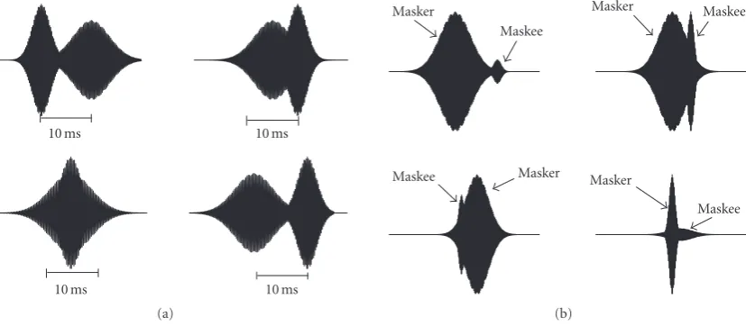
Figure6: (a) Illustration of few possible time occurrences of two TF functions as masker and maskee, (b) possible masking conditions that can occur within the 10 milliseconds time slot.
to 10 milliseconds, the TF functions falling in each time slot were divided into 25 critical bands based on their center fre-quencies. In each critical band, the TF function with high-est energy was located. Relative energy difference of this TF function with the remaining TF functions in the same crit-ical band was computed. Using a lookup table, each of the remaining TF functions was verified if it would be masked by the relative energy difference with the TF function having the highest energy. The experimental procedure for comput-ing the lookup table of maskcomput-ing thresholds will be explained in subsequent paragraphs. The TF functions which fall be-low the masking threshold defined by the lookup tables will be discarded.
As shown inFigure 6(a)within the 10 milliseconds du-ration the location of masker and maskee TF functions can occur anywhere. The worst case situation would be when the masker TF function occurs at the beginning of the time slot, and the maskee TF function occurs at the end of the time slot or vice versa. So all of our testing was done for this worst case scenario by placing the masker TF function and the maskee TF function at the maximum distance of 10 milliseconds.
Based on the duration of masker and maskee TF func-tions, one of the following could occur as depicted in Figure 6(b).
(1) Masker and maskee are apart in time within the 10 mil-liseconds, in which case they do not occur simultane-ously. In this situation masking is achieved due to tem-poral masking effects where a strong occurring masker masks preceding and following weak signals in time domain.
(2) Masker duration is large enough that the maskee du-ration falls within the masker (two scenarios shown in Figure 6(b)) even after a 400 samples shift. In this case, simultaneous masking occurs.
(3) Masker duration is shorter than the maskee duration. In this case, both simultaneous and temporal mask-ings are achieved. The simultaneous masking occurs
during the duration of the masker when the maskee is also present. Temporal masking occurs before and af-ter the duration of the masker.
55 50 45 40 35 30 25 20 15
R
elati
ve
dB
di
ff
er
enc
e
w
ith
mask
er
8 9 10 11 12 13 14
Time width of maskee TF functions 2x Masking curves
Masker freq. Maskee freq. 10500–11250 Hz
10500–12000 Hz
4800–5300 Hz
150–200 Hz 1000–1080 Hz
Figure7: Masking curves for different time width of TF functions.
TF functions and the Y-axis represents the relative energy difference with the masker in dB.
The masking curve obtained for critical band center fre-quency 10.5 kHz deviates from the remaining curves consid-erably. This is due to the fact that the frequency separation between the masker and the maskee becomes very high at this band. This is because we use for all our experiments the up-per limit of the critical band as the maskee frequency to sim-ulate the worst case scenario. To demonstrate this frequency separation dependence on masking performance, a second masking curve was obtained for the critical band with a cen-ter frequency of 10.5 kHz for masker but this time the fre-quency separation between masker and maskee was reduced by half. The curve dropped down explaining the increase in masking performance, that is, when the frequency separation between the masker and maskee was reduced, the average rel-ative dB difference required for masking also reduces.
From these curves it could be observed that the mask-ing curves of critical bands with center frequencies 150 Hz, 1 kHz, and 4.8 kHz remain almost the same. Hence, the masking curve obtained for 1 kHz was used as the lookup table for the first 20 critical bands. The remaining 5 crit-ical bands use the masking curve obtained for the critcrit-ical band with a centre frequency of 10.5 kHz (with 12 kHz up-per limit) as the lookup table. These lookup tables were used to verify if a TF function will be masked by the relative dB difference of it with the TF function having highest energy within the same critical band.
The flow chart inFigure 8gives an overview of the mask-ing implementation used in the proposed coder.
4. QUANTIZATION
Most of the existing transform-based coders rely on con-trolling the quantizer resolution based on psychoacoustic thresholds to achieve compression. Unlike this, the proposed technique achieves a major part of the compression in the transformation itself followed by perceptual filtering. That is,
TF functions
Sort the TF functions into
time slots of 10 ms
TF functions in each time slot are divided into 25 critical bands based on their center frequency
Verification of each TF function with the masking threshold based on lookup tables
Lookup tables
Store index of TF functions
to be removed
Check if all time slots
processed No
Yes Discard the TF
functions & proceed to quantization · · · 25 critical bands· · ·
Figure8: Flow chart of the masking procedure.
when the number of iterationsMneeded to model a signal is very low compared to the length of the signal, we just need M×Lbits. WhereLis the number of bits needed to quantize the 5 TF parameters that represent a TF function. Hence, we limit our research work to scalar quantizers as the focus of the research mainly lies on the TF transformation block and the psychoacoustics block rather than the usual subblocks of the data-compression application.
As explained earlier, each of the five parameters energy (an), centre frequency (fn), time position (pn), octave (sn), and phase (φn) are needed to represent a TF function and thereby the signal itself. These five parameters were to be quantized in such a way that the quantization error intro-duced was imperceptible while, at the same time, obtaining good compression. Each of the five parameters has different characteristics and dynamic range. After careful analysis of them, the following bit allocations were made. In arriving at the final bit allocations informal MOS tests were conducted to compare the quality of the 8 audio samples before and af-ter quantization stage.
In total, 54 bits are needed to represent each TF func-tion without introducing significant perceptual quantizafunc-tion noise in the reconstructed signal. The final form of data for MTF functions will contain the following:
(1) energy parameter (log companded)=M∗12 bits; (2) time position parameter=M∗15 bits;
1 0.9 0.8 0.7 0.6 0.5 0.4 0.3 0.2 0.1 0
Energ
y
(a.u.)
0 50 100 150 200 250 300 350
Number of TF functions Curve-fitted energy curve
Original energy curve
Compressed curve
Figure9: Log companded original and curve-fitted energy curve for a sample signal (au:arbitrary units).
(4) phase parameter=M∗10 bits; (5) octave parameter=M∗4 bits.
The sum of all the above (=54∗M bits) will be the total number of bits transmitted or stored representing an audio segment of duration 5 seconds. The energy parameter after log companding was observed to be a very smooth curve as shown inFigure 9. Fitting a curve to the energy param-eter further reduces the bitrate. Nearly 90% of the energy is present in the first few 100 TF functions and hence they are not used for curve fitting. The remaining number of TF functions is divided into equal lengths of 50 points on the curve. Only the values corresponding to these 50 points need to be sent with the first few original 100 values. The distance between these 50 points can be treated as linear comparing the spread of total number of TF functions. In the recon-struction stage, these 50 points can be interpolated linearly to the original number of points. The error introduced in this procedure was very small due to the smooth slope of the curve. Moreover, this error was introduced only in the 10% energy of the signal which was not perceived. To bet-ter explain the benefit of the proposed curve fitting approach in reducing the bitrate, let us take an example of transmit-ting 5000 TF functions. To transmit the energy parameter for 5000 TF functions (without applying curve fitting) will require 5000∗12 bits = 60 000 bits. With curve fitting, say we preserve the energy parameter for the first 150 TF func-tions and thereafter select the energy parameter from every 50th TF function in the remaining 4850 TF functions. This will result in [150 + (4850/50=97)]=247 values of the en-ergy parameter requiring only 247∗12=2964 bits for trans-mission. We see a massive reduction in bits due to curve fit-ting.Figure 9demonstrates the original curve superimposed with the fitted curve. Everykth point in the compressed curve corresponds to actually the (3 +k)∗50th point in the origi-nal curve. A correlation value of 1 was achieved between the original curve and the interpolated reconstructed curve.
With just a simple scalar quantizer and curve fitting of the energy parameter, the proposed coder achieves high com-pression ratios. Although a scalar quantizer was used to re-duce the computational complexity of the proposed coder, sophisticated vector quantization techniques can be easily in-corporated to further increase the coding efficiency. The 5 parameters of the TF function can be treated as one vec-tor and accordingly quantized using predefined codebooks. Once the vector is quantized, only the index of the codebook needs to be transmitted for each set of TF parameters result-ing in a large reduction of the total number of bits. How-ever, designing the codebooks would be challenging as the dynamic ranges of the 5 TF parameters are drastically diff er-ent. Apart from reducing the number of total bits, the quan-tization stage can also be utilized to control the bitrates suit-able for constant bitrate (CBR) applications.
5. COMPRESSION RATIOS
Compression ratios achieved by the proposed coder were computed for the eight sample signals as described below.
(1) As explained earlier, the total number of bits needed to represent each TF function is 54.
(2) The energy parameter is curve fitted and only the first 150 points in addition to the curve-fitted point need to be coded.
(3) So the total number of bits needed forMiterations for a 5 second duration of the signal isTB1=(M∗42) +
((150 +C)∗12), whereCis the number of curve-fitted points, andMis the number of perceptually important functions.
(4) The total number of bits needed for a CD quality 16 bit PCM technique for a 5 second duration of the signal sampled at 44 100 Hz isTB2 = 44 100∗5∗16 =
3 528 000.
(5) The compression ratio can be expressed as the ratio of the number of bits needed by the proposed coder to the number of bits needed by the CD quality 16 bit PCM technique for the same length of the signal, that is,
Compression ratio=TB2 TB1.
(4)
(6) The overall compression ratio for a signal was then cal-culated by averaging all the 5 seconds duration seg-ments of the signal for both the channels.
that demand network transmissions over constant bitrate channels with limited delays. The proposed coder can also be used in CBR mode by fixing the number of TF functions used for representing signal segments, however due to the signal adaptive nature of the proposed coder, this would compro-mise the quality at instances where signal segments demand a higher number of TF functions for perceptually lossless re-production. Hence, we choose to present the results of the proposed coder using only the VBR mode.
We compare the proposed coder with two existing pop-ular and state-of-the-art audio coders viz MP3 (MPEG 1 layer 3) and MPEG-4 AAC/HE-AAC. Advanced audio cod-ing (AAC) is the current industrial standard which was ini-tially developed for multichannel surround signals (MPEG-2 AAC [16]). The transformation technique used is the mod-ified discrete cosine transform (MDCT). Compared to mp3 which uses a polyphase filter bank and an MDCT, new cod-ing tools were introduced to enhance the performance. The core of MPEG-4 AAC is basically the MPEG-2 AAC but with added tools to incorporate additional coding enhance-ments and MPEG-4 features so that a broad range of appli-cations are covered. There are many application specific pro-files that can be chosen to adaptively configure the MPEG-4 audio for the user needs. It is claimed that at 128 kbps the MPEG-4 AAC is indistinguishable from the original audio signal [17]. As there are ample studies in the literature [9,11, 12,16,18,19] available for both MP3 and MPEG-2/4 AAC, more details about these techniques are not provided in this paper.
As the proposed coder is of VBR type, in our first com-parison we compare the proposed coder with both the MP3 and MPEG-4 AAC coders in VBR mode. All eight sam-ple signals were MP3 coded using the Lame MP3 encoder (version 1.2, Engine 3.88 Alpha 8) in VBR mode [20,21]. For the MPEG-4 AAC, we used the AAC encoder devel-oped by PysTel research (currently ahead software). As there are many profiles possible in AAC, we choose the following suitable profile for our comparison-VBR high quality with main long-term prediction (LTP) [10]. All eight signals were MPEG-4 AAC encoded. The average bitrates for each sig-nal for both MP3 and MPEG-4 AAC was found using the Winamp decoder [22]. These average bitrates were used to calculate the compression ratio as described below.
(1) Bitrate for a CD quality 16 bit PCM technique for 1-second stereo signal is given byTB3=2∗44 100∗16.
(2) The average bitrate/s achieved by (MP3 or MPEG-4 AAC) in VBR mode=TB4.
(3) Compression ratio achieved by (MP3 or MPEG-4 AAC)=TB3/TB4.
The 2nd, 4th, and 6th columns ofTable 1 show the com-pression ratio (CR) achieved by the MP3, MPEG-4 AAC, and the proposed ATFT coders for the set of 8 sample au-dio files. It is evident from the table that the proposed coder has better compression ratios than MP3. When comparing with MPEG-4 AAC, 5 out of 8 signals are either comparable or have better compression ratios than the MPEG-4 AAC. It is noteworthy to mention that for slow music (classical type),
the ATFT coder provides 3 to 4 times better comparison than MPEG-4 AAC or MP3. The compression ratio alone cannot be used to evaluate an audio coder. The compressed audio signals has to undergo a subjective evaluation to compare the quality achieved with respect to the original signal. The combination of the subjective rating and the compression ra-tio will provide a true evaluara-tion of the coder performance. A second comparison was also performed by comparing the HE-AAC profile of the MPEG-4 audio at the same bitrates to that was achieved by the ATFT coder in the VBR mode. More details on the HE-AAC profile of the MPEG-4 audio will be discussed in the subsequent sections. A subjective evaluation was performed as will be explained inSection 6.
Before performing the subjective evaluation, the signal has to be reconstructed. The reconstruction process is a straight forward process of linearly adding all the TF func-tions with their corresponding five TF parameters. In order to do that, first the TF parameters modified for reducing the bitrates have to be expanded back to their original forms. The log-compressed energy curve was log expanded after re-covering back all the curve points using interpolation on the equally placed 50 length points. The energy curve was multi-plied with the normalization factor to bring the energy pa-rameter as it was during the decomposition of the signal. The restored parameters (energy, time-position, centre fre-quency, phase, and octave) were fed to the ATFT algorithm to reconstruct the signal. The reconstructed signal was then smoothed using a third order Savitzky-Golay [23] filter and saved in a playable format.
Figure 10demonstrates a sample signal (/“HARP”/) and its reconstructed version and the corresponding spectro-grams. It can be clearly observed from the reconstructed sig-nal spectrogram compared with the origisig-nal sigsig-nal spectro-gram, how accurately the ATFT technique has filtered out the irrelevant components from the signal (evident from Table 1-(/“HARP”/)-high compression ratio vs. acceptable quality). The accuracy in adaptive filtering of the irrelevant components is made possible by the TF resolution provided by the ATFT algorithm.
6. QUALITY ASSESSMENT OF THE PROPOSED CODER
6.1. Subjective evaluation of ATFT coder
Table1: Compression ratio (CR) and subjective difference grades (SDG). MP3-moving picture experts group I layer 3, AAC-MPEG-4 AAC, moving picture experts group 4 advanced audio coding-VBR main LTP profile, ATFT:adaptive time-frequency transform.
Samples MP3 AAC ATFT
— CR SDG CR SDG CR SDG
ACDC 7.5 0.067 9.3 −0.067 8.4 −0.93
DEFLE 7.7 −0.2 9.5 −0.067 8.3 −1.73
ENYA 9 0 9.6 −0.133 20.6 −0.8
HARP 11 −0.067 9.4 −0.067 36.3 −1
HARPSICHORD 8.5 −0.067 10.2 0.33 9.3 −0.73
PIANO 13.6 0.067 9.6 −0.2 40 −0.8
TUBULARBELL 8.3 0 10.1 0.067 10.5 −0.53
VISIT 8.4 −0.067 11.5 0 11.6 −2.27
Average 9.3 −0.03 9.9 −0.02 18.3 −1.1
0.2 0.1 0 −0.1 −0.2
A
m
plitude
(a.u.)
1 2 3 4
×105
Time samples Original
(a)
×104
2 1.5 1 0.5 0
Fre
q
u
en
cy
(H
z)
0 2 4 6 8
Time (s) Original
(b)
0.2 0.1 0 −0.1 −0.2
A
m
plitude
(a.u.)
1 2 3 4
×105
Time samples Reconstructed
(c)
×104
2 1.5 1 0.5 0
Fre
q
u
en
cy
(H
z)
0 2 4 6 8
Time (s) Reconstructed
(d)
Figure10: Example of a sample original (/“HARP”/) and the reconstructed signal with their respective spectrograms.X-axes for the original and reconstructed signal are in time samples, andX-axes for the spectrogram of the original and the reconstructed signal are in equivalent time in seconds. Note that the sampling frequency=44.1 kHz (au:arbitrary units).
signals with respect to A in 5 levels from 1 to 5. The levels 1 to 5 corresponds to (1) unsatisfactory (or) very annoying, (2) poor (or) annoying, (3) fair (or) slightly annoying, (4) good (or) perceptible but not annoying, and (5) excellent (or) im-perceptible [1,13]. A subjective difference grade (SDG) [1]
is computed by subtracting the absolute score assigned to the hidden reference from the absolute score assigned to the compressed signal. It is given by
Threshold in quiet (TIQ) Wideband
audio
TF modeling
TF parameter
processing Masking Quantizer
Media or channel Perceptual filtering
Reconstructed Reconstructed Reconstructed
A B C
Figure11: Block diagram explaining MOS choices A, B, and C for the subjective evaluation of perceptual filtering and quantization stages.
Table2: Average SDG for PFO and QO (PFO:perceptually filtered output, QO:quantization output).
Samples PFO QO
ACDC −0.8 −0.4
DEFLEP −0.6 −0.6
ENYA −0.8 −1
HARP −0.8 −0.6
HARPSICHORD 0 −0.6
PIANO −0.2 −0.8
TUBULARBELL −0.6 −1.2
VISIT −0.2 −0.4
Average −0.5 −0.7
Accordingly, the scale of SDG will range from (−4 to 0) with the following interpretation, (−4) unsatisfactory (or) very annoying, (−3) poor (or) annoying, (−2) fair (or) slightly annoying, (−1) good (or) perceptible but not an-noying, and (0) excellent (or) imperceptible. Fifteen listen-ers (randomly selected) participated in the MOS studies and evaluated all the 3 audio coders (MP3, AAC, and ATFT in VBR mode). The average SDG was computed for each of the audio sample. The 3rd, 5th, and 7th columns ofTable 1show the SDGs obtained for MP3, AAC, and ATFT coders, respec-tively. MP3 and AAC SDGs fall very close to the Impercepti-ble (0) region, whereas the proposed ATFT SDGs are spread out between−0.53 to−2.27.
A second listening test was performed using the HE-AAC v1/v2 (also known as MPEG-4 HE-AAC v2, HE-AAC PLUS v2) encoder [12]. The HE-AAC encoder is an enhanced high-efficiency version of the AAC with improved audio quality. The HE-AAC v1 encoder comprises of the basic AAC and spectral band replication (SBR) technologies whereas the v2 encoder comprises of AAC, SBR, and parametric stereo (PS) coding technologies. The HE-AAC v2 encoder is rated as the best audio codec at low bitrates. In the second test, SDG were computed for the 8 audio samples by encoding them using HE-AAC v1/v2 coder at the same bitrates/compression ratios as that of the ATFT. Six listeners participated in the second MOS study and the obtained SDG are shown inTable 3. De-tailed discussion of the compression ratio versus subjective evaluation scores is given inSection 7.
6.2. Subjective evaluation of perceptual filtering and quantization stages
In order to evaluate the performance of the developed per-ceptual model and the quantization stage, another listening
test was conducted with 5 listeners. The procedure as de-scribed inSection 6.1was repeated but the choices A, B, and C were assigned as shown in Figure 11. The output of the TF decomposition (TF modeling stage) forms the input to the perceptual filtering module, hence the reference A was assigned to the reconstructed signal at the output of the TF modeling stage. Similarly, choice B was assigned to the re-constructed signal at the output of the perceptual filtering module and C to the reconstructed signal at the output of the quantization stage. Listeners were asked to rate the choices B (perceptual filtering output) and C (quantization stage out-put) with the reference A (TF modeling outout-put) on a scale of 1 to 5 as explained inSection 6.1.
The results were averaged for the five listeners and given inTable 2. FromTable 2, it can be observed on an average, SDGs of −0.5 and −0.7 were achieved for the perceptual filtering stage and the quantization stage, respectively. The SDG scores indicate that the novel perceptual filtering tech-nique proposed is performing exceedingly well with the eight sample signals and the noise introduced in the process of quantization affects the output quality minimally. Interest-ingly, it can be noted fromTable 2 that the signals ACDC, DEFLEP, and VISIT have better SDG scores when the ref-erence is the reconstructed output signal of the TF modeling block than when the reference is the original signal. This gives a valid clue that the low SDG scores achieved by these signals (as seen inTable 1) are not due to the perceptual filtering or the quantization stages but may be due to TF modeling with symmetrical type Gaussian functions.
7. RESULTS AND DISCUSSION
7.1. Performance comparison in VBR mode
The compression ratios (CR) and the SDG for all three coders (MP3, AAC, and ATFT) are shown inTable 1. All the coders were tested in the VBR mode. For the proposed tech-nique, VBR was the best way to present the performance ben-efit of using an adaptive decomposition approach. In ATFT, the type of the signal and the characteristics of the TF func-tions (type of dictionary) control the number of transfor-mation parameters required to approximate the signal and thereby the compression ratio. The inherent variability intro-duced in the number of TF functions required to model a sig-nal is one of the highlights of using ATFT. Hence, we choose to present comparison of the coders in the VBR mode.
Table3: SDG comparison of MPEG-4 AAC PLUS coder for the same compression ratio/bitrate achieved by the proposed ATFT coder. Modes: 1. HE-high efficiency AAC v1 (AAC and spectral band replication (SBR)) and 2. HEv2-high efficiency AAC v2 (AAC, SBR and parametric stereo (PS) coding).
Samples HE-AAC v1/2 ATFT
— MODE Kbps CR SDG SDG
ACDC HE 168 8.4 0.17 −0.93
DEFLE HE 170 8.3 0.17 −1.73
ENYA HEv2 68 20.6 −0.17 −0.8
HARP HEv2 38 36.3 0 −1
HARPSICHORD HE 151 9.3 −0.33 −0.73
PIANO HEv2 35 40 0.17 −0.8
TUBULARBELL HE 134 10.5 0 −0.53
VISIT HE 121 11.6 0.33 −2.27
Average — 111 18.3 0.04 −1.1
45 40 35 30 25 20 15 10 5
C
o
mpr
ession
ra
tio
(CR)
−4 −3 −2 −1 0 1
MP3 AAC ATFT
Very annoying Imperceptible
Subjective difference grade (SDG)
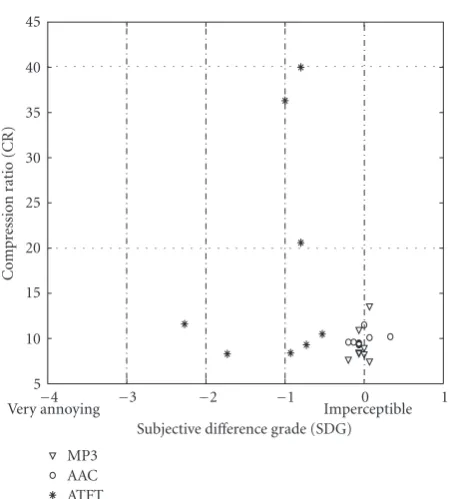
Figure12: Subjective difference grade (SDG) versus compression ratios (CR).
compression ratio around 10. The proposed coder does not perform well with all of the eight samples. Out of the 8 samples, 6 samples have an SDG between −0.53 to −1 (imperceptible-perceptible but not annoying) and 2 samples have SDG below−1. Out of the 6 samples with SDGs be-tween (−0.53 and −1), 3 samples (ENYA, HARP, and PI-ANO) have compression ratios 2 to 4 times higher than MP3 and AAC and 3 samples (ACDC, HARPSICHORD, and TUBULARBELL) have comparable compression ratios with moderate SDGs.
Figure 12shows the comparison of all three coders by plotting the samples with their SDGs inX-axis and compres-sion ratios in theY-axis. If we can virtually divide this plot
in segments of SDGs (horizontally) and the compression ra-tios (vertically), then the ideal desirable coder performance should be in the right top corner of the plot (high compres-sion ratios and excellent SDG scores). This is followed next by the right bottom corner (low compression ratios and ex-cellent SDG scores) and so on as we move from right to left in the plot. Here, the terms “low” and “high” compression ratios are used in a relative sense based on the compression ratios achieved by all the 3 coders in this study. From the plot it can be seen the MP3 and AAC coders occupy the right bot-tom corner, whereas the samples from ATFT coder are spread over. As mentioned earlier, 3 out the 8 samples of the ATFT coder occupy the right top corner however only with mod-erate SDGs that are much less than the MP3 and the AAC. Three out of the remaining 5 samples of the ATFT coder oc-cupy the right bottom corner, however again with only mod-erate SDGs that are less than MP3 and AAC. The remain-ing 2 samples perform the worst occupyremain-ing the left bottom corner.
lowest of the group−2.27. The poor performances with the two audio sample cases could be addressed by using a hybrid dictionary of TF functions and residue coding the noncoher-ent structures separately. However, this would increase the computational complexity of the coder and reduce the com-pression ratios.
7.2. Performance comparison with same bitrates (high-efficiency AAC)
In the second performance comparison of the ATFT coder, we choose to test the high-efficiency profile of the MPEG-4 AAC v2 at the same bitrates as that of the ATFT coder. As per [12], the HE-AAC v2 improves the coding gain of the AAC by 4 times and outperforms most of the existing coders in audio quality especially at low bitrates. All the 8 samples were encoded using the HE-AAC v1/v2 encoder at the same bitrates as that of the VBR bitrates of the ATFT. The choice for the v1 or the v2 encoder was determined by the target bi-trates (below 70 kbps v2 was used). From the SDGs obtained as shown inTable 3, it is very evident that the HE-AAC pro-files of the MPEG-4 audio codec outperforms the proposed ATFT coder for the same bitrates. However, it would not be fair to compare the HE-AAC directly with the ATFT, since ATFT is a basic coder without the additional enhancements achieved by SBR or any form of parametric coding.
Although we did not include standalone sinusoidal coders in our comparison, the MPEG-4 HE-AAC v2 in-cludes the parametric stereo coding based on the transient-sinusoid-noise (TSN) model and is derived from the MPEG-4 audio sinusoidal coding (also abbreviated as SSC) [25]. The TSN model though in existence for quite some time for audio and speech coding, received much attention recently with its inclusion in the MPEG-4 audio standard for low-bitrate ap-plications. The formal verification tests of the MPEG-4 SSC indicate that the SSC coder performs either comparable to or better than 4 AAC even at lower bitrates than MPEG-4 AAC [25]. Another recent well-known family of sinusoidal codec (the SiCAS codec and its variants) is from the research group of Heusdens et al. and Philips Research Laboratories [26]. It is shown that the psychoacoustics model used in this family of codecs is better than the MPEG I Layer I-II psy-choacoustics model [27]. The subjective listening tests indi-cate that this family of codec performs equal to or better than MPEG-4 at low bitrates (16 Kbps (HILN), 24 Kbps (SSC), and 32 Kbps (AAC)) [26]. Various improvements have been proposed for this codec family over the years with an in-cremental performance gain [28,29]. Interestingly, the im-provements proposed in using amplitude modulated sinu-soids over constant amplitude sinusinu-soids indicate the migra-tion of these approaches towards completely adaptive signal decompositions such as the one proposed in the ATFT coder [29].
8. CONCLUSIONS
This paper presented a novel ATFT coding technique for wideband audio signals. The proposed approach
demon-strated the application of adaptive time-frequency transform for audio coding and the development of a novel psychoa-coustics model adapted to TF functions. The compression strategy was changed from the conventional way of control-ling quantizer resolution to achieving majority of the com-pression in the transformation itself. Eight stereo sample sig-nals were used in the study. Listening tests were conducted and the performance comparison of the proposed coder with MP3 and AAC coders was presented. From the preliminary results, although the proposed coder achieves high com-pression ratios, its SDG scores are well below the MP3 and AAC family of coders. The proposed coder however performs moderately well for slowly varying classical-like signals with acceptable SDGs. The proposed coder is not as refined as the state-of-the-art commercial coders, which to some extent ex-plains its poor performance. Future work involves testing the proposed coder with a hybrid dictionary of TF functions and including professional refinements.
REFERENCES
[1] T. Painter and A. Spanias, “Perceptual coding of digital audio,” Proceedings of the IEEE, vol. 88, no. 4, pp. 451–515, 2000. [2] S. G. Mallat and Z. Zhang, “Matching pursuits with
time-frequency dictionaries,”IEEE Transactions on Signal Process-ing, vol. 41, no. 12, pp. 3397–3415, 1993.
[3] K. Umapathy and S. Krishnan, “Joint time-frequency coding of audio signals,” inProceedings of the 5th WSES/IEEE Multi-conference on Circuits, Systems, Communications, and Comput-ers (CSCC ’01), pp. 32–36, Crete, Greece, July 2001.
[4] K. Umapathy and S. Krishnan, “Low bit-rate coding of wide-band audio signals,” inProceedings of IASTED International Conference on Signal Processing, Pattern Recognition and Appli-cations (SPPRA ’01), pp. 101–105, Rhodes, Greece, July 2001. [5] R. Heusdens, R. Vafin, and W. B. Kleijn, “Sinusoidal modeling
using psychoacoustic-adaptive matching pursuits,”IEEE Sig-nal Processing Letters, vol. 9, no. 8, pp. 262–265, 2002. [6] T. S. Verma and T. H. Y. Meng, “Sinusoidal modeling
us-ing frame-based perceptually weighted matchus-ing pursuits,” inProceedings of IEEE International Conference on Acoustics, Speech and Signal Processing (ICASSP ’99), vol. 2, pp. 981–984, Phoenix, Ariz, USA, March 1999.
[7] R. Heusdens, J. Jensen, P. Korten, and R. Vafin, “Rate-distortion optimal high-resolution differential quantisation for sinusoidal coding of audio and speech,” inIEEE Workshop on Applications of Signal Processing to Audio and Acoustics (AS-PAA ’05), pp. 243–246, New Paltz, NY, USA, October 2005. [8] R. Heusdens and J. Jensen, “Jointly optimal time
segmen-tation, component selection and quantization for sinusoidal coding of audio and speech,” in Proceedings of IEEE Inter-national Conference on Acoustics, Speech and Signal Process-ing (ICASSP ’05), vol. 3, pp. 193–196, Philadelphia, Pa, USA, March 2005.
[9] I. JTC1/SC29/WG11, “Overview of the MPEG-4 standard,” in International Organization for Standardisation, March 2002. [10] J. Herre and B. Grill, “Overview of MPEG-4 audio and its
ap-plications in mobile communications,” inProceedings of the 5th International Conference on Signal Processing (ICSP ’00), vol. 1, pp. 11–20, Beijing, China, August 2000.
[12] S. Meltzer and G. Moser, “MPEG-4 HE-AAC v2—audio cod-ing for today’s digital media world,” Tech. Rep., EBU Technical Review, Geneva, Switzerland, January 2006.
[13] T. Ryden, “Using listening tests to assess audio codecs,” in Col-lected Papers on Digital Audio Bit Rate Reduction, N. Gilchrist and C. Grewin, Eds., pp. 115–125, Audio Engineering Society, New York, NY, USA, 1996.
[14] S. Mallat,A wavelet Tour of Signal Processing, Academic Press, San Diego, Calif, USA, 1998.
[15] L. Cohen, “Time-frequency distributions: a review,” Proceed-ings of the IEEE, vol. 77, no. 7, pp. 941–981, 1989.
[16] K. Brandenburg and M. Bosi, “MPEG-2 advanced audio cod-ing: overview and applications,” inThe 103rd Audio Engineer-ing Society Convention, p. 4641, Ney York, NY, USA, August 1997.
[17] http://www.apple.com/MPEG4/aac/.
[18] E. Eberlein and H. Popp, “Layer-3, a flexible coding standard,” inThe 94th Audio Engineering Society Convention, p. 3493, Berlin, Germany, March 1993.
[19] http://www.iis.fraunhofer.de/bf/amm/. [20] http://lame.sourceforge.net/index.php. [21] http://www.mp3dev.org/.
[22] http://www.winamp.com/.
[23] S. J. Orfanidis,Introduction to Signal Processing, Prentice-Hall, Englewood Cliffs, NJ, USA, 1996.
[24] M. M. Goodwin,Adaptive Signal Models: Theory, Algorithms and Audio Applications, Kluwer Academic Publishers, Boston, Mass, USA, 1998.
[25] ISO/IEC JTC 1/SC 29/WG 11N6675, “Report on the verifica-tion tests of MPEG-4 parametric coding for high quality au-dio,” in International Organization for Standardisation, July 2004.
[26] R. Heusdens, J. Jensen, W. B. Kleijn, et al., “Bit-rate scalable intraframe sinusoidal audio coding based on rate-distortion optimization,”Journal of the Audio Engineering Society, vol. 54, no. 3, pp. 167–188, 2006.
[27] S. van de Par, A. Kohlrausch, R. Heusdens, J. Jensen, and S. H. Jensen, “A perceptual model for sinusoidal audio coding based on spectral integration,”EURASIP Journal on Applied Signal Processing, vol. 2005, no. 9, pp. 1292–1304, 2005.
[28] P. Korten, J. Jensen, and R. Heusdens, “High-resolution spher-ical quantization of sinusoidal parameters,”IEEE Transactions on Audio, Speech, and Language Processing, vol. 15, no. 3, pp. 966–981, 2007.