Eigenmode analysis of the electromagnetic ﬁeld scattered by an elliptic cone

(1)

Adv. Radio Sci., 9, 31–37, 2011 www.adv-radio-sci.net/9/31/2011/ doi:10.5194/ars-9-31-2011

Advances in

Radio Science

Eigenmode analysis of the electromagnetic field scattered by an

elliptic cone

M. Kijowski and L. Klinkenbusch

Institute of Electrical and Information Engineering, Christian-Albrechts-Universit¨at zu Kiel, Germany

Abstract. The vector spherical-multipole analysis is applied

to determine the scattering of a plane electromagnetic wave by a perfectly electrically conducting (PEC) semi-infinite el-liptic cone. From the eigenfunction expansion of the total field in the space outside the elliptic cone, the scattered far field is obtained as a multipole expansion of the free-space type by a single integration over the induced surface cur-rents. As for the evaluation of the free-space-type expansion it is necessary to apply suitable series transformation tech-niques, a sufficient number of eigenfunctions has to be con-sidered. The eigenvalues of the underlying two-parametric eigenvalue problem with two coupled Lam´e equations be-long to the Dirichlet- or the Neumann condition and can be arranged as so-called eigenvalue curves. It has been observed that the eigenvalues are in two different domains: In the first one Dirichlet- and Neumann eigenvalues are either nearly co-inciding, while in the second one they are strictly separated. The eigenfunctions of the first (coinciding) type look very similar to free-space modes and do not contribute to the scat-tered field. This observation allows to significantly improve the determination of diffraction coefficients.

1 Introduction

Electromagnetic scattering by a PEC elliptic cone is of prac-tical importance for several reasons. First, the geometry in-cludes a tip, and the related tip-diffraction coefficient could be used to improve asymptotically valid methods like GTD and UTD in describing scattering by complex electrically large systems. Second, as the geometry can be treated mostly analytically using sphero-conal coordinates and the vector spherical-multipole expansion, the obtained results (e.g., for

Correspondence to: L. Klinkenbusch ([email protected])

a finite elliptic cone with the degenerations sector and cir-cular cone) can serve as a reference for numerical com-putations. Scattering by circular and (less often) by ellip-tic cones have been treated by many authors in the litera-ture. Summaries on the different approaches can be found in Bowman et al. (1987); Klinkenbusch (2007). This paper starts with a description of sphero-conal coordinates which are used to describe the elliptic cone geometry. For an inci-dent plane electromagnetic wave the exact total field outside and the corresponding surface current on the elliptic cone are determined by a spherical-multipole (eigenfunction) expan-sion based on suitable solutions of the scalar homogeneous Helmholtz equation. The far field is then found as a free-space type spherical-multipole expansion from an integra-tion over the surface current. In sphero-conal coordinates the solution of the scalar Helmholtz equation leads to a two-parametric eigenvalue problem with two coupled Lam´e dif-ferential equations, that is, the difdif-ferential equations of the periodic and of the non-periodic Lam´e functions. The two separation parameters can be arranged on so-called eigen-value curves on which the Dirichlet- and Neumann eigenval-ues are discretely distributed. It turns out that the numeri-cal determination of some of these eigenvalues is difficult, however, as will be shown exactly these eigenvalues do not significantly contribute to the scattered far field and can be automatically sorted out. Finally, this procedure leads to an improved accuracy in determining the scattering coefficient magnitudes and phases.

(2)

32 M. Kijowski and L. Klinkenbusch: Eigenmode analysis of the field scattered by an elliptic cone

2 M. Kijowski and L. Klinkenbusch: Eigenmode analysis of the field scattered by an elliptic cone

ϑx

y

ϑ

z y

x

k = 0.52

ϑ=ϑ0

r=r₀

0

ϕ=ϕ

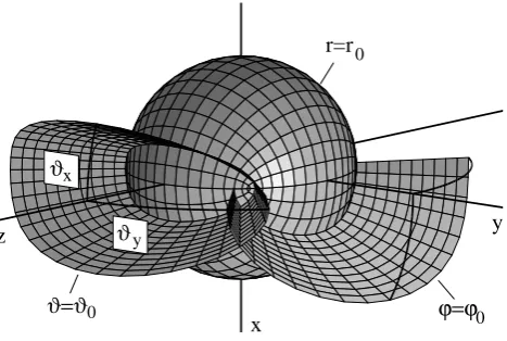
Fig. 1. Sphero-conal coordinate surfaces

The ranges of the values are

0 _≤

r <

_∞

,

0 _≤

ϑ

_≤

π

,

0 _≤

ϕ

_≤

2 π

and the ellipticity parameters k and k’ satisfy

0 _≤

k, k

′

≤

1;

k

2

+

k

′2

= 1

.

(2)

The coordinate surfaces are shown in Fig. 1. The elliptic

cone is identical to the coordinate surface

ϑ

=

ϑ

0

and can be

characterized by the half opening angles

ϑ

x

=

ϑ

0

and

ϑ

y

=

arccos(

k

cos

ϑ

0

)

. The normalized metric scaling coefficients

are given by

s

ϑ

=

1 r

∂

r

∂ϑ

=

s

k

2

_sin

2

_ϑ

₊

_k

′₂

cos

2

_ϕ

1 ₋

k

2

_cos

2

_ϑ

(3)

s

ϕ

=

1 r

∂

r

∂ϕ

=

s

k

2

sin

2

ϑ

+

k

′2

cos

2

ϕ

1 ₋

k

′2

_sin

2

_ϕ

(4)

Note that the elliptic cone includes several interesting

de-generations: For

k

= 1

the elliptic cone turns into a

circu-lar cone while

ϑ

0

=

π

describes a plane angular sector with

half-opening angle

arccos(

k

)

.

3 Eigenfunction Expansion of the Total Field

In a linear, homogeneous, and isotropic domain outside the

elliptic cone the total electromagnetic field can be derived as

a multipole (eigenfunction) expansion in sphero-conal

coor-dinates which is based on the corresponding solution of the

scalar homogeneous Helmholtz equation

∆Ψ(

r

_{) +}

_κ

2

_Ψ(

r

_{) = 0}

₍₅₎

where

κ

=

ω

√

µε

denotes the wave number. A first

separa-tion ansatz

Ψ(

r,ϑ,ϕ

) =

R

(

r

)

Y

(

ϑ,ϕ

)

(6)

with a first separation constant

ν

(

ν

+ 1)

leads to the

differen-tial equation of the spherical Bessel functions with solutions

z

ν

(

κr

)

and to the eigenvalue equation of surface spherical

harmonics which are referred to as Lam´e products in case of

sphero-conal coordinates

(

r

_×

∇

₎

2

_Y

_ν

₍

_ϑ,ϕ

_{) +}

_ν

₍

_ν

_{+ 1)}

_Y

_ν

₍

_ϑ,ϕ

_{) = 0}

₍₇₎

For the given problem it is necessary to have solutions which

are (at least)

2 π

- periodic in

ϕ

and fulfill canonical boundary

conditions at

ϑ

=

ϑ

0

:

Dirichlet condition:

Y

σ

(

ϑ,ϕ

)

|

ϑ=ϑ0

= 0

(8)

Neumann condition:

∂Y

τ

(

ϑ,ϕ

)

∂ϑ

ϑ=ϑ0

= 0

(9)

A second separation ansatz of the form

Y

ν

(

ϑ,ϕ

) = Θ

ν

(

ϑ

)Φ

ν

(

ϕ

)

(10)

with a second separation constant

λ

yields two ordinary

dif-ferential equations:

q

1 ₋

k

′2

_sin

2

_ϕ

d

dϕ

q

1 ₋

k

′2

_sin

2

_ϕ

d

Φ

ν

dϕ

+

λ

₋

ν

(

ν

+ 1)

k

′2

sin

2

ϕ

Φ

ν

= 0

(11)

p

1 ₋

k

2

_cos

2

_ϑ

d

dϑ

p

1 ₋

k

2

_cos

2

_ϑ

d

Θ

ν

dϑ

+

ν

(

ν

+ 1)(1

₋

k

2

cos

2

ϑ

)

₋

λ

Θ

ν

= 0

(12)

Equation (11) is referred to as the differential equation of the

periodic Lam´e functions

Φ

ν

(

ϕ

)

while Eq. (12) represents

the differential equation of the non-periodic Lam´e functions

Θ

ν

(

ϑ

)

. The periodic Lam´e functions can be described as

in-finite Fourier series and the non-periodic Lam´e functions are

expanded into infinite series using associated Legendre

func-tions of the 1st kind (Boersma and Jansen, 1990). In case

of solutions in the free unbounded space the eigenvalues are

integers (

ν

=

n

= 1

,

2 ,

3 ,..

), the series become finite, and

con-sequently the solutions turn into periodic and non-periodic

Lam´e polynomials

Φ

nm

(

ϕ

)

and

Θ

nm

(

ϑ

)

, respectively.

For a given value of

ν

and of the parameter

k

2

the

cor-responding second separation constant

λ

can be numerically

determined. The resulting

(

ν,λ

)

-pairs lie on characteristic

eigenvalue curves sorted by numbers

m

= 0

,

1 ,

2 ,..

.

Any

arbitrary pair of eigenvalues

(

ν,λ

)

lying on the eigenvalue

curves leads to a valid solution of the eigenvalue equation of

the Lam´e products (7). Additional Dirichlet- and Neumann

boundary conditions imposed upon the nonperiodic Lam´e

functions

Θ

ν

at

ϑ

0

result in a discrete spectrum of eigenvalue

pairs

(

ν

i

,λ

i

)

(

i

= 1

,

2 ,

3 ,..

) lying on the eigenvalue curves.

Figure 2 exemplarily shows the eigenvalue curves with

dis-crete Dirichlet- and Neumann eigenvalues. Due to the

Sturm-Liouville properties of the Lam´e differential equations the

discrete Dirichlet- and Neumann eigenvalues strictly must

al-ternate on the eigenvalue curves (Boersma and Jansen, 1990).

Outside the PEC elliptic cone the total

electromag-netic field can be expressed in the form of a

spherical-multipole (eigenfunction) expansion (Stratton, 1941; Blume

Fig. 1. Sphero-conal coordinate surfaces.

2 Sphero-conal coordinates

Sphero-conal coordinatesr,ϑ,ϕare related to Cartesian co-ordinates by (Boersma and Jansen, 1990)

x=rsinϑcosϕ y=r

√

1−k2_cos2_ϑ_sin_ϕ

z=rcosϑ

q

1−k02_sin2_ϕ

(1)

The ranges of the values are 0≤r <∞, 0≤ϑ≤π, 0≤

ϕ≤2πand the ellipticity parameterskandk0satisfy

0≤k, k0≤1; k2+k02=1. (2)

The coordinate surfaces are shown in Fig. 1. The elliptic cone is identical to the coordinate surfaceϑ=ϑ0and can be characterized by the half opening anglesϑx=ϑ0andϑy=

arccos(kcosϑ0). The normalized metric scaling coefficients are given by

sϑ=

1

r

∂r

∂ϑ

=

s

k2sin2ϑ+k02cos2ϕ

1−k2_cos2_ϑ (3)

sϕ=

1

r

∂r

∂ϕ

=

s

k2sin2ϑ+k02cos2ϕ

1−k02_sin2_ϕ (4)

Note that the elliptic cone includes several interesting de-generations: Fork=1 the elliptic cone turns into a circu-lar cone whileϑ0=πdescribes a plane angular sector with half-opening angle arccos(k).

3 Eigenfunction expansion of the total field

In a linear, homogeneous, and isotropic domain outside the elliptic cone the total electromagnetic field can be derived as a multipole (eigenfunction) expansion in sphero-conal coor-dinates which is based on the corresponding solution of the scalar homogeneous Helmholtz equation

19(r)+κ29(r)=0 (5) whereκ=ω√µεdenotes the wave number. A first separa-tion ansatz

9(r,ϑ,ϕ)=R(r)Y (ϑ,ϕ) (6) with a first separation constantν(ν+1)leads to the differen-tial equation of the spherical Bessel functions with solutions

zν(κr) and to the eigenvalue equation of surface spherical

harmonics which are referred to as Lam´e products in case of sphero-conal coordinates

(r×∇)2Yν(ϑ,ϕ)+ν(ν+1)Yν(ϑ,ϕ)=0 (7)

For the given problem it is necessary to have solutions which are (at least) 2π– periodic inϕand fulfill canonical boundary conditions atϑ=ϑ0:

Dirichlet condition: Yσ(ϑ,ϕ)|ϑ=ϑ0=0 (8)

Neumann condition: ∂Yτ(ϑ,ϕ)

∂ϑ

_ϑ₌_ϑ

0

=0 (9)

A second separation ansatz of the form

Yν(ϑ,ϕ)=2ν(ϑ )8ν(ϕ) (10)

with a second separation constantλyields two ordinary dif-ferential equations:

q

1−k02_sin2_ϕ d

dϕ

q

1−k02_sin2_ϕd8ν

dϕ

+hλ−ν(ν+1)k02sin2ϕi8ν=0 (11)

p

1−k2_cos2_ϑ d

dϑ

p

1−k2_cos2_ϑd2ν

dϑ

+hν(ν+1)(1−k2cos2ϑ )−λi2ν=0 (12)

Equation (11) is referred to as the differential equation of the periodic Lam´e functions8ν(ϕ)while Eq. (12) represents

the differential equation of the non-periodic Lam´e functions

2ν(ϑ ). The periodic Lam´e functions can be described as

in-finite Fourier series and the non-periodic Lam´e functions are expanded into infinite series using associated Legendre func-tions of the 1st kind (Boersma and Jansen, 1990). In case of solutions in the free unbounded space the eigenvalues are in-tegers (ν=n=1,2,3,..), the series become finite, and con-sequently the solutions turn into periodic and non-periodic Lam´e polynomials8nm(ϕ)and2nm(ϑ ), respectively.

For a given value of ν and of the parameterk2 the cor-responding second separation constantλcan be numerically determined. The resulting(ν,λ)-pairs lie on characteristic eigenvalue curves sorted by numbersm=0,1,2,... Any arbi-trary pair of eigenvalues(ν,λ)lying on the eigenvalue curves

(3)

M. Kijowski and L. Klinkenbusch: Eigenmode analysis of the field scattered by an elliptic cone 33

M. Kijowski and L. Klinkenbusch: Eigenmode analysis of the field scattered by an elliptic cone

3

0 5 10 15 20 25 30 35 40

0 200 400 600 800 1000 1200 1400 1600 1800

ν λ

Dirichlet Neumann

Fig. 2. Eigenvalue curvesλ(ν)fork2= 0.5with Dirichlet eigen-values (×) and Neumann eigenvalues (◦)

and Klinkenbusch, 1999)

E

tot

₍

r

_{) =}

X

σ

a

σ

N

σ

(

r

) +

Z

j

X

τ

b

τ

M

τ

(

r

)

(13)

H

tot

₍

r

_{) =}

j

Z

X

σ

a

σ

M

σ

(

r

) +

X

τ

b

τ

N

τ

(

r

)

(14)

where the expansion functions which are referred to as the

vector spherical-multipole functions can be derived from the

elementary solutions of the scalar homogeneous Helmholtz

equation

Ψ

ν

(

r

)

by

M

_ν

₍

r

_{) = (}

r

_×

∇

_)Ψ

_ν

₍

r

₎

=

z

ν

(

κr

)

m

ν

(

ϑ,ϕ

)

(15)

N

_ν

₍

r

_{) =}

1 κ

[

∇

×

(

r

×

∇

)]Ψ

ν

(

r

)

=

₋

z

ν

(

κr

)

κr

n

(

n

+ 1)

Y

ν

(

ϑ,ϕ

)ˆ

r

−

_κr

1 _dr

d

[

rz

ν

(

κr

)]

n

ν

(

ϑ,ϕ

)

(16)

with

r

ˆ

=

r

_/r

_{denoting the unit vector and}

_κ

₌

_ω

√

_ε

₀

_µ

₀

_being

the wave number in the free space. The transverse vector

functions are defined as

m

_ν

₍

_ϑ,ϕ

_{) =}

₋

1 s

ϕ

∂Y

ν

(

ϑ,ϕ

)

∂ϕ

ϑ

ˆ

+

1 s

ϑ

∂Y

ν

(

ϑ,ϕ

)

∂ϑ

ϕ

ˆ

(17)

n

_ν

₍

_ϑ,ϕ

_{) =}

1 s

ϑ

∂Y

ν

(

ϑ,ϕ

)

∂ϕ

ϑ

ˆ

+

1 s

ϕ

∂Y

ν

(

ϑ,ϕ

)

∂ϑ

ϕ

ˆ

(18)

and the electric and magnetic multipole amplitudes are given

by

a

σ

and

b

τ

, respectively. Note that the indices

σ

and

τ

symbolize the Dirichlet- and Neumann conditions as defined

in (8) and (9) to ensure the vanishing of the tangential

elec-tric field on the surface of the PEC elliptic cone. The

inci-dent plane wave is realized by locating a Hertzian dipole at

infinity and multiplying the resulting field by an appropriate

factor (Blume and Klinkenbusch, 1999). For a plane wave

with amplitude

E

0

incident from

(

θ

inc

,φ

inc

)

and electrically

polarized in the direction

C, the multipole amplitudes of the

ˆ

total field are found as

α

σ

= 4

πE

0

e

j(σ+1)π

2

σ

(

σ

+ 1)

[

n

σ

· C

ˆ

]

(19)

β

τ

= 4

π

E

0

Z

e

j(τ+1)π

2

τ

(

τ

+ 1)

[

m

τ

· C

ˆ

]

(20)

where

Z

=

p

µ

0

/ε

0

is the intrinsic impedance of the free

space.

4 Spherical-Multipole Expansion of the Scattered Field

The scattered field is determined from the surface current

J

_S

₌

₋

_ϑ

ˆ

_×

H

tot

_|

ϑ0

on the cone’s surface by

E

₍

r

_{) =}

Z

V

Γ

0

(

r

,

r

′

)

· J

s

(

r

′

)

dv

′

(21)

where the dyadic Green’s function of the free space in

bilin-ear form is deduced as

Γ

0

(

r

,

r

′

) =

(22)

jκ

X

n,m

N

II

n,m

(

r

)

N

In,m

(

r

′

)

n

(

n

+ 1)

+

jκ

X

n,m

M

II

n,m

(

r

)

M

In,m

(

r

′

)

n

(

n

+ 1)

At a time-factor

e

jωt

_{the upper indices}

_I

_and

_II

_{stand for the}

use of spherical Bessel functions of the first kind (z

n

=

j

n

)

and of spherical Hankel functions of the second kind (z

n

=

h

(2)n

), respectively. It has been shown (Klinkenbusch, 2006)

that the scattered electric far field can be written in form of a

multipole expansion

E

sc

₍

r

_{) =}

e

−jκr

κr

"

−

X

n,m

a

sc

n,m

j

n

n,m

+

X

n,m

Z

j

b

sc

n,m

j

n+1

m

n,m

#

(23)

Fig. 2. Eigenvalue curvesλ(ν)fork2=0.5 with Dirichlet eigenval-ues (×) and Neumann eigenvalues (◦).

leads to a valid solution of the eigenvalue equation of the Lam´e products Eq. (7). Additional Dirichlet- and Neumann boundary conditions imposed upon the non-periodic Lam´e functions2νatϑ0result in a discrete spectrum of eigenvalue pairs(νi,λi)(i=1,2,3,..) lying on the eigenvalue curves.

Figure 2 exemplarily shows the eigenvalue curves with dis-crete Dirichlet- and Neumann eigenvalues. Due to the Sturm-Liouville properties of the Lam´e differential equations the discrete Dirichlet- and Neumann eigenvalues strictly must al-ternate on the eigenvalue curves (Boersma and Jansen, 1990). Outside the PEC elliptic cone the total electromag-netic field can be expressed in the form of a spherical-multipole (eigenfunction) expansion (Stratton, 1941; Blume and Klinkenbusch, 1999)

Etot(r)=X

σ

aσNσ(r)+

Z j

X

τ

bτMτ(r) (13)

Htot(r)= j

Z

X

σ

aσMσ(r)+

X

τ

bτNτ(r) (14)

where the expansion functions which are referred to as the vector spherical-multipole functions can be derived from the elementary solutions of the scalar homogeneous Helmholtz equation9ν(r)by

Mν(r)=(r×∇)9ν(r)

=zν(κr)mν(ϑ,ϕ) (15)

Nν(r)=

1

κ[∇×(r×∇)]9ν(r)

= −zν(κr)

κr n(n+1)Yν(ϑ,ϕ)rˆ

− 1

κr d

dr[rzν(κr)]nν(ϑ,ϕ) (16)

withrˆ=r/rdenoting the unit vector andκ=ω√ε0µ0being the wave number in the free space. The transverse vector functions are defined as

mν(ϑ,ϕ)= −

1

sϕ

∂Yν(ϑ,ϕ)

∂ϕ

ˆ

ϑ+ 1

sϑ

∂Yν(ϑ,ϕ)

∂ϑ ϕˆ (17)

nν(ϑ,ϕ)=

1

sϑ

∂Yν(ϑ,ϕ)

∂ϕ

ˆ

ϑ+ 1

sϕ

∂Yν(ϑ,ϕ)

∂ϑ ϕˆ (18)

and the electric and magnetic multipole amplitudes are given byaσ andbτ, respectively. Note that the indices σ andτ

symbolize the Dirichlet- and Neumann conditions as defined in Eqs. (8) and (9) to ensure the vanishing of the tangential electric field on the surface of the PEC elliptic cone. The in-cident plane wave is realized by locating a Hertzian dipole at infinity and multiplying the resulting field by an appropriate factor (Blume and Klinkenbusch, 1999). For a plane wave with amplitudeE0incident from(θinc,φinc)and electrically polarized in the directionCˆ, the multipole amplitudes of the total field are found as

ασ =4π E0

ej (σ+1)π2

σ (σ+1)[nσ· ˆC] (19) βτ =4π

E0

Z

ej (τ+1)π2

τ (τ+1)[mτ· ˆC] (20)

where Z=√µ0/ε0 is the intrinsic impedance of the free space.

4 Spherical-multipole expansion of the scattered field

The scattered field is determined from the surface current

JS= − ˆϑ×Htot

ϑ0 on the cone’s surface by

E(r)= Z

V

00(r,r0)·Js(r0)dv0 (21)

where the dyadic Green’s function of the free space in bilin-ear form is deduced as

00(r,r0)= (22)

j κX

n,m

NI I_n,m(r)NI_n,m(r0₎

n(n+1) +j κ

X

n,m

MI I_n,m(r)MI_n,m(r0₎

n(n+1)

At a time-factorej ωtthe upper indicesIandI Istand for the use of spherical Bessel functions of the first kind (zn=jn)

and of spherical Hankel functions of the second kind (zn=

h(n2)), respectively. It has been shown (Klinkenbusch, 2006)

that the scattered electric far field can be written in form of a multipole expansion

Esc(r)=

e−j κr κr

"

−X

n,m

asc_n,mjnnn,m+

X

n,m

Z jb

sc n,mjn

+1_m

n,m

#

(23) with the multipole amplitudes

(4)

4 M. Kijowski and L. Klinkenbusch: Eigenmode analysis of the field scattered by an elliptic cone

with the multipole amplitudes

a

scn,m

=

−

j

Θ

n,m

(

ϑ

0

)

(

p

1 ₋

k

2

_cos

2

_ϑ

0

X

σ

α

σ

d

Θ

σ

dϑ

_ϑ 0 ∞

Z

0

j

n

(

κr

)

r

j

σ

(

κr

)

κrdr

2π

Z

0

Φ

n,m

(

ϕ

)Φ

σ

(

ϕ

)

p

1 ₋

k

′₂

_sin

2

_ϕ

dϕ

−

X

τ

Z

j

β

τ

Θ

τ

(

ϑ

0

)

∞

Z

0

j

n

(

κr

)

r

[

rj

τ

(

κr

)]

′

κr

κrdr

2π

Z

0

Φ

n,m

(

ϕ

)

d

Φ

τ

(

ϕ

)

dϕ

+

X

τ

Z

j

β

τ

Θ

τ

(

ϑ

0

)

τ

(

τ

+ 1)

n

(

n

+ 1)

∞

Z

0

[

rj

n

(

κr

)]

′

κr

j

τ

(

κr

)

r

κrdr

2π

Z

0

d

Φ

n,m

(

ϕ

)

dϕ

Φ

τ

(

ϕ

)

dϕ

)

(24)

Z

j

b

sc n,m

=

j

d

Θ

n,m

dϑ

_ϑ 0

p

1 ₋

k

2

_cos

2

_ϑ

0

X

τ

Z

j

β

τ

Θ

τ

(

ϑ

0

)

τ

(

τ

+ 1)

n

(

n

+ 1)

∞

Z

0

j

n

(

κr

)

j

τ

(

κr

)

r

κrdr

2π

Z

0

Φ

n,m

(

ϕ

)Φ

τ

(

ϕ

)

p

1 ₋

k

′₂

_sin

2

_ϕ

dϕ.

(25)

Finally, the scattered far field can be written as a function of

the incident field by means of a scattering matrix as

E

sc θ

(

θ,φ

)

E

sc

φ

(

θ,φ

)

=

e

−jκr

κr

D

θθ

D

θφ

D

φθ

D

φφ

E

inc θ

(

θ

′

,φ

′

)

E

inc φ

(

θ

′

,φ

′

)

(26)

While the series in (24) and (25) converge and yield stable

multipole amplitudes of the scattered field, the resulting

se-ries in (23) do not converge. In order to obtain a meaningful

limiting value it is necessary to apply a suitable sequence

transformation. In contrast to nonlinear techniques (like the

Shanks transform) linear sequence transformations always

yield consistent results. For the linear Ces`aro transform the

transformed partial sum sequence

s

′

n

is obtained from the

original partial sum sequence

s

n

by

s

′

n

=

s

0

+

s

1

+

s

2

+

...

+

s

n

+ 1

, n

= 0

,

1 ,

2 ,..

(27)

The sequence transformation can be repeatedly applied to

enforce faster convergence of the resulting partial sum

se-quence. Figure 3 shows the double transformed partial sum

sequence of the scattering coefficent

D

θθ

as a function of

n. Clearly, a higher order of the original series and hence a

higher number of eigenvalues is desired to obtain more

ac-curate results. In order to increase the maximum number of

0 5 10 15 20 25 30 35 40

−2 −1 0 1 2 3 n Re(D θθ ) original 1x Cesaro 2x Cesaro

Fig. 3. Partial sum sequence of the real part of the scattering

coef-ficientDθθ for the maximum order ofnmax= 40. Dotted curve is original partial sum sequence, dashed curve is single Ces`aro trans-formed sequence and solid curve is double Ces`aro transtrans-formed se-quence.

available eigenvalues and eigenfunctions it is necessary to

in-vestigate the relevance of eigenvalues and eigenmodes which

will be sketched in the following section.

5 Eigenmode analysis

In Fig. 2 it has been shown that the discrete

(

ν,λ

)

-pairs

ar-ranged in an eigenvalue-curve scheme which can

approxi-mately be divided into an upper region where Dirichlet- and

Neumann eigenvalues nearly coincide and into a lower

re-gion where Dirichlet- and Neumann eigenvalues are strictly

20 22 24 26 28 30

200 250 300 350 400 450 500 ν λ Dirichlet Neumann

Fig. 4. Detailed view of the eigenvalue curves of Lam´e functions

fork2

= 0.5with Dirichlet- (×) and Neumann (◦) eigenvalues.

coef-ficientDθ θ for the maximum order ofnmax=40. Dotted curve is original partial sum sequence, dashed curve is single Ces`aro trans-formed sequence and solid curve is double Ces`aro transtrans-formed se-quence.

asc_n,m= −j 2n,m(ϑ0)

p

1−k2cos2_ϑ 0 X σ ασ d2σ dϑ ϑ0 ∞ Z 0

jn(κr)

r jσ(κr)κrdr

2π

Z

0

8n,m(ϕ)8σ(ϕ)

q

1−k02_sin2_ϕ

dϕ

−X

τ

Z

jβτ2τ(ϑ0)

∞

Z

0

jn(κr)

r

[rjτ(κr)]0

κr κrdr

2π

Z

0

8n,m(ϕ)

d8τ(ϕ)

dϕ dϕ

+X

τ

Z

jβτ2τ(ϑ0)

τ (τ+1) n(n+1)

∞

Z

0

[rjn(κr)]0

κr

jτ(κr)

r κrdr

2π

Z

0

d8n,m(ϕ)

dϕ 8τ(ϕ)dϕ

(24)

Z j b

sc n,m=j

d2n,m dϑ ϑ0 p

1−k2_cos2_ϑ 0

X

τ

Z

j βτ2τ(ϑ0)

τ (τ+1) n(n+1)

∞

Z

0

jn(κr)

jτ(κr)

r κrdr

2π

Z

0

8n,m(ϕ)8τ(ϕ)

q

1−k02_sin2_ϕ

dϕ.

(25)

4 M. Kijowski and L. Klinkenbusch: Eigenmode analysis of the field scattered by an elliptic cone

with the multipole amplitudes

a

sc_n,m

=

₋

j

Θ

n,m

(

ϑ

0

)

(

p

1 ₋

k

2

_cos

2

_ϑ

0

X

σ

α

σ

d

Θ

σ

dϑ

_ϑ 0 ∞

Z

0

j

n

(

κr

)

r

j

σ

(

κr

)

κrdr

2π

Z

0

Φ

n,m

(

ϕ

)Φ

σ

(

ϕ

)

p

1 ₋

k

′₂

_sin

2

_ϕ

dϕ

−

X

τ

Z

j

β

τ

Θ

τ

(

ϑ

0

)

∞

Z

0

j

n

(

κr

)

r

[

rj

τ

(

κr

)]

′

κr

κrdr

2π

Z

0

Φ

n,m

(

ϕ

)

d

Φ

τ

(

ϕ

)

dϕ

+

X

τ

Z

j

β

τ

Θ

τ

(

ϑ

0

)

τ

(

τ

+ 1)

n

(

n

+ 1)

∞

Z

0

[

rj

n

(

κr

)]

′

κr

j

τ

(

κr

)

r

κrdr

2π

Z

0

d

Φ

n,m

(

ϕ

)

dϕ

Φ

τ

(

ϕ

)

dϕ

)

(24)

Z

j

b

sc

n,m

=

j

d

Θ

n,m

dϑ

_ϑ 0

p

1 ₋

k

2

_cos

2

_ϑ

0

X

τ

Z

j

β

τ

Θ

τ

(

ϑ

0

)

τ

(

τ

+ 1)

n

(

n

+ 1)

∞

Z

0

j

n

(

κr

)

j

τ

(

κr

)

r

κrdr

2π

Z

0

Φ

n,m

(

ϕ

)Φ

τ

(

ϕ

)

p

1 ₋

k

′₂

_sin

2

_ϕ

dϕ.

(25)

Finally, the scattered far field can be written as a function of

the incident field by means of a scattering matrix as

E

sc

θ

(

θ,φ

)

E

sc

φ

(

θ,φ

)

=

e

−jκr

κr

D

θθ

D

θφ

D

φθ

D

φφ

E

inc

θ

(

θ

′

,φ

′

)

E

inc

φ

(

θ

′

,φ

′

)

(26)

While the series in (24) and (25) converge and yield stable

multipole amplitudes of the scattered field, the resulting

se-ries in (23) do not converge. In order to obtain a meaningful

limiting value it is necessary to apply a suitable sequence

transformation. In contrast to nonlinear techniques (like the

Shanks transform) linear sequence transformations always

yield consistent results. For the linear Ces`aro transform the

transformed partial sum sequence

s

′

n

is obtained from the

original partial sum sequence

s

n

by

s

′

n

=

s

0

+

s

1

+

s

2

+

...

+

s

n

+ 1

, n

= 0

,

1 ,

2 ,..

(27)

The sequence transformation can be repeatedly applied to

enforce faster convergence of the resulting partial sum

se-quence. Figure 3 shows the double transformed partial sum

sequence of the scattering coefficent

D

θθ

as a function of

n. Clearly, a higher order of the original series and hence a

higher number of eigenvalues is desired to obtain more

ac-curate results. In order to increase the maximum number of

0 5 10 15 20 25 30 35 40

−2 −1 0 1 2 3 n Re(D θθ ) original 1x Cesaro 2x Cesaro

coef-ficientDθθfor the maximum order ofnmax= 40. Dotted curve is original partial sum sequence, dashed curve is single Ces`aro trans-formed sequence and solid curve is double Ces`aro transtrans-formed se-quence.

available eigenvalues and eigenfunctions it is necessary to

in-vestigate the relevance of eigenvalues and eigenmodes which

will be sketched in the following section.

5 Eigenmode analysis

In Fig. 2 it has been shown that the discrete

(

ν,λ

)

-pairs

ar-ranged in an eigenvalue-curve scheme which can

approxi-mately be divided into an upper region where Dirichlet- and

Neumann eigenvalues nearly coincide and into a lower

re-gion where Dirichlet- and Neumann eigenvalues are strictly

20 22 24 26 28 30

200 250 300 350 400 450 500 ν λ Dirichlet Neumann

fork2= 0.5with Dirichlet- (×) and Neumann (◦) eigenvalues.

fork2=0.5 with Dirichlet- (×) and Neumann (◦) eigenvalues.

Finally, the scattered far field can be written as a function of the incident field by means of a scattering matrix as

E_θsc(θ,φ) E_φsc(θ,φ)

=e

−j κr

κr

Dθ θ Dθ φ

Dφθ Dφφ

E_θinc(θ0,φ0) E_φinc(θ0,φ0)

(26) While the series in Eqs. (24) and (25) converge and yield stable multipole amplitudes of the scattered field, the result-ing series in Eq. (23) do not converge. In order to obtain a meaningful limiting value it is necessary to apply a suitable sequence transformation. In contrast to nonlinear techniques (like the Shanks transform) linear sequence transformations always yield consistent results. For the linear Ces`aro trans-form the transtrans-formed partial sum sequence s_n0 is obtained from the original partial sum sequencesnby

s_n0=s0+s1+s2+...+sn

n+1 , n=0,1,2,.. (27) The sequence transformation can be repeatedly applied to enforce faster convergence of the resulting partial sum se-quence. Figure 3 shows the double transformed partial sum sequence of the scattering coefficentDθ θ as a function of

n. Clearly, a higher order of the original series and hence a higher number of eigenvalues is desired to obtain more ac-curate results. In order to increase the maximum number of available eigenvalues and eigenfunctions it is necessary to in-vestigate the relevance of eigenvalues and eigenmodes which will be sketched in the following section.

5 Eigenmode analysis

In Fig. 2 it has been shown that the discrete(ν,λ)-pairs ar-ranged in an eigenvalue-curve scheme which can approxi-mately be divided into an upper region where Dirichlet- and

(5)

M. Kijowski and L. Klinkenbusch: Eigenmode analysis of the field scattered by an elliptic cone

5

0 50 100 150 200 −0.5

0 0.5

ν=20.00000184750623 λ=352.44290601629518

ϑ [deg]

Θν

(

ϑ

)

0 50 100 150 200 0

0.2 0.4

ν=18.00000000486987 λ=329.29483207551141

ϑ [deg]

Θν

(ϑ

)

0 50 100 150 200 −0.5

0 0.5

ν=25.00582154305340 λ=423.23802115275748

ϑ [deg]

Θν

(

ϑ

)

0 50 100 150 200 −1

0 1

ν=38.49087220085550 λ=740.18392974181609

ϑ [deg]

Θν

(

ϑ

)

0 50 100 150 200 −0.5

0 0.5

ν=55.71295858579171 λ=1204.87393839763990

ϑ [deg]

Θν

(ϑ

)

0 50 100 150 200 −0.4

−0.2 0

n=18, m=10(10)

ϑ [deg]

Θn

(ϑ

)

0 50 100 150 200 −0.5

0 0.5

n=20, m=10(11)

ϑ [deg]

Θn

(ϑ

)

0 50 100 150 200 −0.5

0 0.5

n=25, m=10(13)

ϑ [deg]

Θn

(

ϑ

)

0 50 100 150 200 −0.5

0 0.5

n=38, m=11(20)

ϑ [deg]

Θn

(

ϑ

)

0 50 100 150 200 −0.5

0 0.5

n=56, m=10(29)

ϑ [deg]

Θn

(

ϑ

)

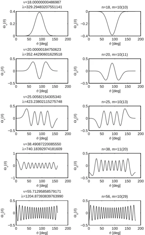
Fig. 5. Sequence of non-periodic Lam´e functions Θν(ϑ) to the Dirichlet boundary condition atϑ0= 160◦,k

2

= 0.5(left column) and (corresponding) non-periodic Lam´e polynomialsΘn(ϑ)(right column), each as function of the arguments.

separated. Figure 4 shows a closer view of this phenomenon

revealing that the coinciding eigenvalues all are very near to

integral values (integers) of

ν

. Since the numerical

computa-tion of these coinciding eigenvalues turns out to imply some

numerical difficulties limiting the maximum number of

com-putable eigenvalues we will now investigate that case in more

detail.

The left column in Fig. 5 shows a sequence of plots of

non-periodic Lam´e functions each satisfying the Dirichlet

bound-ary condition at

ϑ

0

= 160

◦

as a function of the argument

ϑ

. In

the right column we see plots of the non-periodic Lam´e

poly-nomials (with integral eigenvalues

ν

=

n

) at (

n,λ

)-pairs on

the same eigenvalue curve nearest by those ones of the

corre-sponding non-periodic Lam´e functions. We observe that for

nearly integral eigenvalues of the non-periodic Lam´e

func-tions not only their values at

ϑ

0

are vanishing but also their

derivatives. Moreover, these eigenfunctions look very

simi-lar to the corresponding non-periodic Lam´e polynomials. At

non-integral eigenvalues only the values of the non-periodic

Lam´e functions vanish but not their derivatives, and their

curves are different from the corresponding non-periodic

Lam´e polynomials, at least in the vicinity of the boundaries

ϑ

= 0

and

ϑ

=

π

. This general behavior is typical and can be

observed for any other eigenvalue as well.

Due to numerical reasons, the computation of the nearly

integral eigenvalues and -functions turns out to be difficult.

However, as we can deduce from the representations of the

multipole amplitudes (24) and (25) the modes belonging to

these eigenvalues do not significantly contribute to the

scat-tered far field. Each part of (24) and (25) has a factor of one

of the following forms

Θ

τ

(

ϑ

0

)

(28)

d

Θ

σ

(

ϑ

)

dϑ

ϑ=ϑ0

(29)

Clearly, if both function and derivative of a non-periodic

Lam´e function are small at

ϑ

0

, the corresponding scattering

mode is also small compared to the other scattering modes.

In other words, these eigenmodes of the PEC cone do not

sig-nificantly lead to a surface current on the cone, or, the cone

is nearly invisible for these eigenmodes. Consequently, they

are very similar to free-space modes, which are characterized

by integral eigenvalues.

Following this observation, these nearly-integral

eigenval-ues and eigenfunctions don’t need to be exactly calculated,

and the modified algorithm allows to calculate much more

relevant eigenvalues and eigenfunctions to come to more

ac-curate scattering coefficients.

6 Scattering coefficients

Figure 6 shows the amplitude and the phase of the electric

far field scattered by a PEC semi-infinite elliptic cone

illumi-nated by a plane wave electrically polarized in the xz plane

and incident from

θ

inc

_{= 105}

◦

,

φ

inc

_{= 0}

◦

. The amplitude of

the scattering coefficient

D

θθ

is shown for the maximum

or-der

n

max

= 40

including the integral-eigenvalue modes and

n

max

= 60

excluding these non-contributing modes. The

comparison between the phases shows marginal differences,

however, the differences in amplitudes reveal the

improve-ment of the results by considering more relevant eigenmodes.

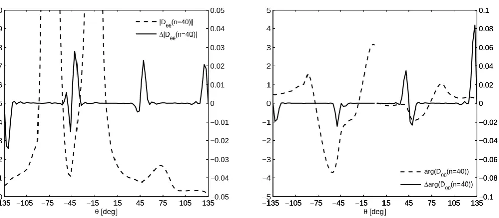
Finally, Fig. 7 proves that the errors of amplitudes and

phases of the scattering coefficient are actually marginal

when all of the near-integer eigenvalues are neglected.

7 Conclusions

It has been found that the accuracy of computed scattering

coefficients for a PEC elliptic cone can be greatly improved if

Fig. 5. Sequence of non-periodic Lam´e functions2ν(ϑ ) to the

Dirichlet boundary condition atϑ₀=160◦,k2=0.5 (left column) and (corresponding) non-periodic Lam´e polynomials2n(ϑ )(right

column), each as function of the arguments.

Neumann eigenvalues nearly coincide and into a lower re-gion where Dirichlet- and Neumann eigenvalues are strictly separated. Figure 4 shows a closer view of this phenomenon revealing that the coinciding eigenvalues all are very near to integral values (integers) ofν. Since the numerical computa-tion of these coinciding eigenvalues turns out to imply some numerical difficulties limiting the maximum number of com-putable eigenvalues we will now investigate that case in more detail.

The left column in Fig. 5 shows a sequence of plots of non-periodic Lamé functions each satisfying the Dirichlet bound-ary condition atϑ0=160◦as a function of the argumentϑ. In the right column we see plots of the non-periodic Lamé polynomials (with integral eigenvaluesν=n) at (n,λ)-pairs on the same eigenvalue curve nearest by those ones of the corresponding non-periodic Lamé functions.

We observe that for nearly integral eigenvalues of the non-periodic Lamé functions not only their values atϑ0are van-ishing but also their derivatives. Moreover, these eigenfunc-tions look very similar to the corresponding non-periodic Lamé polynomials. At non-integral eigenvalues only the values of the non-periodic Lamé functions vanish but not their derivatives, and their curves are different from the cor-responding non-periodic Lamé polynomials, at least in the vicinity of the boundariesϑ=0 andϑ=π. This general be-havior is typical and can be observed for any other eigenvalue as well.

Due to numerical reasons, the computation of the nearly integral eigenvalues and -functions turns out to be difficult. However, as we can deduce from the representations of the multipole amplitudes Eqs. (24) and (25) the modes belong-ing to these eigenvalues do not significantly contribute to the scattered far field. Each part of Eqs. (24) and (25) has a factor of one of the following forms

2τ(ϑ0)

d2σ(ϑ )

dϑ

_ϑ₌_ϑ

0

Clearly, if both function and derivative of a non-periodic Lam´e function are small atϑ0, the corresponding scattering mode is also small compared to the other scattering modes. In other words, these eigenmodes of the PEC cone do not sig-nificantly lead to a surface current on the cone, or, the cone is nearly invisible for these eigenmodes. Consequently, they are very similar to free-space modes, which are characterized by integral eigenvalues.

Following this observation, these nearly-integral eigenval-ues and eigenfunctions don’t need to be exactly calculated, and the modified algorithm allows to calculate much more relevant eigenvalues and eigenfunctions to come to more ac-curate scattering coefficients.

6 Scattering coefficients

Figure 6 shows the amplitude and the phase of the electric far field scattered by a PEC semi-infinite elliptic cone illumi-nated by a plane wave electrically polarized in the xz plane and incident fromθinc=105◦,φinc=0◦. The amplitude of the scattering coefficientDθ θ is shown for the maximum

or-dernmax=40 including the integral-eigenvalue modes and

nmax=60 excluding these non-contributing modes. The comparison between the phases shows marginal differences, however, the differences in amplitudes reveal the improve-ment of the results by considering more relevant eigenmodes. Finally, Fig. 7 proves that the errors of amplitudes and phases of the scattering coefficient are actually marginal when all of the near-integer eigenvalues are neglected.

(6)

−135 −1050 −75 −45 −15 15 45 75 105 135 10

20 30 40 50 60

θ [deg]

|D_θθ(n=60)|

|D_θθ(n=40)|

−135 −105 −75 −45 −15 15 45 75 105 135 −5

−4 −3 −2 −1 0 1 2 3 4 5

θ [deg]

arg(D_θθ(n=60))

arg(D_θθ(n=40))

Fig. 6. Amplitude and phase of the scattering coefficientDθθin the xz plane of a PEC semi-infinite elliptic cone with the half opening angles

αx= 45◦,αy= 60◦for the order of the multipole expansion (23)nmax= 40(dashed line) andnmax= 60(solid line). The plane wave is

incident fromθinc= 105◦_,_φinc_{= 0}◦_.

−135 −1050 −75 −45 −15 15 45 75 105 135 1

2 3 4 5 6 7 8 9 10

θ [deg]

|D_θθ(n=40)| ∆|D_θθ(n=40)|

−135 −105 −75 −45 −15 15 45 75 105 135−0.05 −0.04 −0.03 −0.02 −0.01 0 0.01 0.02 0.03 0.04 0.05

−135 −105−5 −75 −45 −15 15 45 75 105 135 −4

−3 −2 −1 0 1 2 3 4 5

θ [deg]

arg(D_θθ(n=40)) ∆arg(D_θθ(n=40))

−135 −105 −75 −45 −15 15 45 75 105 135−0.1 −0.08 −0.06 −0.04 −0.02 0 0.02 0.04 0.06 0.08 0.1

Fig. 7. Amplitude and phase of the scattering coefficientDθθ(dashed line) in the xz plane of a PEC semi-infinite elliptic cone with the half

opening anglesαx= 45◦,αy= 60◦andnmax= 40. The plane wave is incident fromθinc= 105◦,φinc= 0◦. The solid line using the right

scale is the difference between the first amplitude (phase) resulting from all eigenvalues and the second amplitude (phase) resulting from all eigenvalues except nearly integer eigenvalues.

Fig. 6. Amplitude and phase of the scattering coefficientDθ θin the xz plane of a PEC semi-infinite elliptic cone with the half opening angles

αx=45◦,αy=60◦for the order of the multipole expansion (23)nmax=40 (dashed line) andnmax=60 (solid line). The plane wave is incident fromθinc=105◦,φinc=0◦.

−135 −1050 −75 −45 −15 15 45 75 105 135 10

20 30 40 50 60

θ [deg]

|D_θθ(n=60)|

|D_θθ(n=40)|

−135 −105 −75 −45 −15 15 45 75 105 135 −5

−4 −3 −2 −1 0 1 2 3 4 5

θ [deg]

arg(D θθ(n=60)) arg(D

θθ(n=40))

Fig. 6. Amplitude and phase of the scattering coefficientDθθin the xz plane of a PEC semi-infinite elliptic cone with the half opening angles

αx= 45◦,αy= 60◦for the order of the multipole expansion (23)nmax= 40(dashed line) andnmax= 60(solid line). The plane wave is

incident fromθinc

= 105◦_,_φinc = 0◦_.

−135 −1050 −75 −45 −15 15 45 75 105 135 1

2 3 4 5 6 7 8 9 10

θ [deg]

|D_θθ(n=40)| ∆|D_θθ(n=40)|

−135 −105 −75 −45 −15 15 45 75 105 135−0.05 −0.04 −0.03 −0.02 −0.01 0 0.01 0.02 0.03 0.04 0.05

−135 −105 −75 −45 −15 15 45 75 105 135 −5

−4 −3 −2 −1 0 1 2 3 4 5

θ [deg]

arg(D_θθ(n=40)) ∆arg(D

θθ(n=40))

−135 −105 −75 −45 −15 15 45 75 105 135−0.1 −0.08 −0.06 −0.04 −0.02 0 0.02 0.04 0.06 0.08 0.1

Fig. 7. Amplitude and phase of the scattering coefficientDθθ(dashed line) in the xz plane of a PEC semi-infinite elliptic cone with the half

opening anglesαx= 45◦,αy= 60◦andnmax= 40. The plane wave is incident fromθinc= 105◦,φinc= 0◦. The solid line using the right

scale is the difference between the first amplitude (phase) resulting from all eigenvalues and the second amplitude (phase) resulting from all eigenvalues except nearly integer eigenvalues.

Fig. 7. Amplitude and phase of the scattering coefficientDθ θ (dashed line) in the xz plane of a PEC semi-infinite elliptic cone with the half

opening anglesαx=45◦,αy=60◦andnmax=40. The plane wave is incident fromθinc=105◦,φinc=0◦. The solid line using the right scale is the difference between the first amplitude (phase) resulting from all eigenvalues and the second amplitude (phase) resulting from all eigenvalues except nearly integer eigenvalues.

(7)

7 Conclusions

It has been found that the accuracy of computed scattering coefficients for a PEC elliptic cone can be greatly improved if computationally difficult but non-relevant modes of the scat-tered field are neglected. These non-scatscat-tered modes have nearly integral eigenvalues and are very similar to the free-space modes of the incident field. Further work will include an investigation into the nature of these non-scattered modes. Acknowledgements. This work was supported by the Deutsche

Forschungsgemeinschaft (DFG).

References

Blume, S. and Klinkenbusch, L.: Spherical-multipole analysis in electromagnetics, in: Frontiers in Electromagnetics, edited by: Werner, D. H. and Mittra, R., 553–606, IEEE Press, New York, 1999.

Boersma, J. and Jansen, J. K. M.: Electromagnetic field singulari-ties at the tip of an elliptic cone, EUT-Report 90-WSK-01, Fac-ulty of Mathematics and Computing Science, Eindhoven Univer-sity of Technology, Eindhoven, 1990.

Bowman, J. J., Senior, T. B. A., and Uslenghi, P. L. E.: Electromag-netic and acoustic scattering by simple shapes (Revised Printing), Hemisphere Pub. Corp., New York, 1987.

Klinkenbusch, L.: Modal Analysis of the GTD Diffraction Coeffi-cients for the Half-Plane’s Edge, Electr. Eng., 88, 337–342, 2006. Klinkenbusch, L.: Electromagnetic scattering by semi-infinite circular and elliptic cones, Radio Sci., 42, RS6S10, doi:10.1029/2007RS003649, 2007.

Magnus, W., Oberhettinger, F., and Soni, R. P.: Formulas and theo-rems for the special functions of mathematical physics, Springer-Verlag, New York, 1966.

Stratton, J. A.: Electromagnetic Theory, McGraw-Hill, New York, 1941.