R E S E A R C H
Open Access
Numerical approach for airframe assembly
simulation
Margarita V Petukhova
1*, Sergey V Lupuleac
1, Yulia K Shinder
1, Alexander B Smirnov
1, Sergey
A Yakunin
1and Bertrand Bretagnol
2*Correspondence:
[email protected] 1Department of Applied
Mathematics, Saint Petersburg State Polytechnic University, Saint Petersburg, Russian Federation Full list of author information is available at the end of the article
Abstract
Purpose:The paper describes the methodology of contact problem solving that is used for simulation of aircraft assembly process.
Methods:The dimension of the problem is reduced after eliminating the unknowns outside the contact zone and the initial problem transforms into the problem of quadratic programming with linear constraints.
Results:The special computer code ASRP (Assembly Simulation of Riveting Process) was developed on the base of presented methodology. Now this code is utilized by Airbus. Some results of application of developed code are given in this paper.
Keywords: contact problem; riveting process; quadratic programming; dimension reduction
1 Introduction
Usually the components of the airframe (fuselage sections, wings etc.) are produced in different plants and joined together in Final Assembly Line (FAL) (Figure ). The assembly of an airframe in FAL takes up to a week. This process is one of the bottlenecks for speed-up the overall aircraft production rate. So the optimization and acceleration of assembly process is one of the most urgent problems for aircraft building companies.
All main parts of the airframe are joined together by riveting. The assembly process is rather complicated and consists of several stages:
. The parts to be assembled are brought together and initial clamping is performed. . The holes in assembled parts are drilled sequentially and temporary fasteners are
installed in these holes. After completion of this stage the initial gap needs to be closed.
. The temporary assembly is examined and shimming is performed if needed. . The temporary fasteners are removed, the assembly is taken apart, the parts are
cleaned and sealant layer is applied.
. The assembly is fastened again by temporary fasteners.
. Sequentially the temporary fasteners are removed, the holes are widened and permanent rivets are installed in their positions.
During the assembly process it is important to control both gap between joined parts and stresses caused by installed fasteners. On the one hand tight contact between parts should be achieved; on the other hand engineers should avoid cracks, composite layer separation and part destruction.
Figure 1 Assembly of Airbus A380.
Figure 2 Considered model.Three panels (green, purple and blue ones) are joined together. Maximum possible contact zone is shown in red.
The main goal of the presented work is to develop special tool which allows engineers to perform simulations in order to evaluate displacements and stresses of aircraft parts on the assembly line. For this purpose ASRP software complex was developed for solving special class of contact problems that particularly arise during the simulation of riveting process. Let us denote this class as classR. The considered classRhas specific features that were taken into account during construction of problem solving technique:
• The area where contact may occur is known apriori and is relatively small regarding whole model. Further we will refer to it as junction area.
• Tangential displacements are negligibly small in comparison with the normal ones in the junction area.
• External loads are applied in the junction area or can be transferred there. • Friction is not taken into account.
• Stress state of each considered body obeys linear theory of elasticity. • The problem is considered as stationary.
• Usually it is necessary to perform the number of numerical experiments (e.g. with different fastener arrangements or initial gaps) on the same mechanical model. The developed ASRP complex considerably surpasses commercial FEM codes in speed and user convenience for simulation of aircraft assembly process.
The structure and features of this software are described in [] and [].
The present paper gives the detailed description of developed mathematical algorithm as well as application examples.
2 Main section
2.1 Methodology for gap computations
Let us consider finite element model representing several panels to be assembled (as it is shown in Figure ). These panels overlap in so called junction area shown by red lines. The contact between panels is possible only inside the junction area.
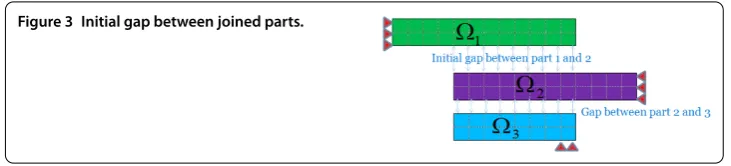
Initially panels are separated by distance called initial gap (see Figure ).
Figure 3 Initial gap between joined parts.
If we do not take into account possibility of contact between panels, the determination of{Uj}Mj=needs only solving the system of linear equations:
K·U=F, ()
whereK={kij}Mi,j=is global stiffness matrix,F={fj}Mj=is vector of loads.
Also it is necessary to impose the boundary conditions to avoid rigid body motion:
Uj=Uj, xj∈Uh, ()
whereUhis a part of the boundary where displacements are specified.
The system (), () is supplemented with following restriction to avoid interpenetration of the panels:
(A·U)j≤G(xj), xj∈Ch. ()
HereAis linear operator determining the relative displacement of parts in normal direc-tion,G(xj) is a function of normal initial gap in the nodexj;Chis junction area that is the
set of nodes that can come into contact.
To finalize problem statement we pose conditions on contact stresses: in the contact points the normal stresses are contradirectional and have the same value. For classRthe friction between parts is not taken into account, so tangential stresses in contact points are zero. Thus we consider so-called unilateral contact problem. As it was shown in [], the solution of this problem provides good agreement with aircraft assembly experiment. The equivalent variational formulation is used to determine the displacements. The dis-placement vector{Uj}Mj=under the loadF={fj}Mj=provides minimum to the energy func-tional
E(U) = U
T·K·U–FT·U ()
on the set of all admissible displacementsAC:
AC={U|U=UinUh,A·U≤GinCh}. ()
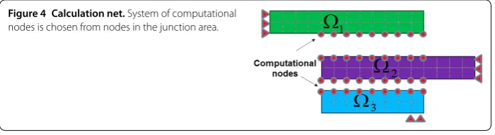
Figure 4 Calculation net.System of computational nodes is chosen from nodes in the junction area.
Further in the paragraph we are to formulate the reduced minimization problem (with unknowns in junction area) equivalent to () and ().
For that we choose the system of computational nodesCN= (cn,cn, . . . ,cnl) in junction
area, for example, as in Figure (lis the total number of nodes in junction area). We denote it calculation net. It consists of nodes where displacements will be computed. We will build the reduced rigidity matrix KC, which allows to pass from whole model to calculation
net.
Reduced rigidity matrix characterizes the response of computational nodes to the ap-plied load. To be more precise,K–
C ={kij}li,j=is inverse matrix toKCandkijis a
displace-ment ofjth node caused by the unit load applied toith computational node. Let us consider a method for computing matrixKC.
We divide whole displacement vector into two parts:U=UC
UR
, whereUCis vector of
displacements in junction area,URis vector of displacements in all other nodes.
Then global stiffness matrixK from () can be written in blocks, and system () trans-forms to
KCC KCR
KCRT KRR
· UC UR = FC FR . ()
Calculating Schur complement for the blockKRR(see []) we obtain reduced rigidity
ma-trixKCinstead of blockKCC.
Also this matrix can be computed using the formula:
KC=KCC–KCR·KRR–·KCRT. ()
Reduced rigidity matrix is computed once for considered junction during data prepara-tion stage. Then this matrix is stored and can be used for series of computaprepara-tions because changes of initial gap or applied loads do not affectKC. This computational decomposition
is relevant for simulation of riveting process as it is aimed at solving variety of problems with different fastener configurations and different relative positions of joined parts.
Now we can formulate equivalent minimization problem forUC:
min
UC∈AC
U
T
C·KC·UC–FCT·UC
, ()
whereAC={UC|A·UC≤G}.
The rest of displacementsURare recovered by the following relation:
UR= –KRR–·KCRT ·UC. ()
It is not difficult to prove that vectorU= (UCUR)Tis a solution of minimization problem
() and () if and only ifUC is a solution of the problem () andUR is determined by
equation ().
Problem () is a quadratic programming problem (QPP). The method for its solution is discussed in the next section.
The solving of problem () gives us the field of displacements in junction areaUCas well
as contact forces obtained as Lagrange multipliers. If we are interested in complete field of displacementsU, we can add the relations
Uj=UCj, xj∈Ch, ()
to the system (), () and solve the obtained system of linear equations. Or alternatively we add contact forces to the vector of loadsFand also solve the system (), () to obtainU. Knowing field of displacements, it is easy to obtain all information about deformed-stress state of our system (including strains and stresses).
Also it is possible to use more refined finite element model to find field of stresses within considered algorithm. To do so we interpolate the computed displacements and/or contact forces to the refined mesh and then compute stresses using linear static analysis.
2.2 Quadratic programming problem solving .. Problem statement
In this section we consider the algorithm used for solving QPP () and its adaptation to the peculiarities of contact problems from classR.
In () matrixKCis ill-conditioned. Moreover, it is symmetric and positive-definite. If we
consider riveting process of n parts, then vectorUCis constructed from displacements of
nodes on each part independent of each other:
UCT=UCT,UCT, . . . ,UCnT, ()
whereUT
Ciis a vector of displacements in contact nodes ofith part.
For such a vector of displacements full reduced rigidity matrix takes a following appear-ance:
KC=
⎛ ⎜ ⎜ ⎜ ⎝
KC · · ·
KC · · ·
· · · ·
· · · KCn
⎞ ⎟ ⎟ ⎟
⎠, ()
From () one can see that matrixKChas block diagonal structure.
MatrixAthat defines admissible set in problem () has a simple structure: each row of matrixAcontains one or two non-zero elements. It is due to the fact that node-to-node contact is considered. Thus constraint matrixAcan be considered as sparse matrix.
.. Algorithm description
We made a review of algorithms for solving QPP: interior point methods, gradient projec-tion methods and active set methods. The last group meets our goals as iteraprojec-tion process finishes after finite number of steps and algorithms allow to simply vary initial approxi-mation. One of the most popular algorithms for solving QPP is described in [, ]. It is known as Goldfarb-Idnani algorithm with Powell modification and is used in this project (further it is called G-I-P). Goldfarb-Idnani active set method is proved to be fast and effi-cient; furthermore the Powell modification is favorable for ill-conditioned problems. This method is also implemented in well-known libraries such as IMSL Numerical Library and Scilab for solving quadratic programming problem.
The main idea of considered algorithm is:
• To start at the point of unconstrained minimum of the problem. If it satisfies the constraints (there is no contact in junction area), then this is desired solution.
• If the constraints are violated, the iteration procedure starts. At each iteration step the current point is forced to satisfy one of violated constraints in a way:
(A·UC)i=Gi, i= ,n. ()
• It is done until the point is in admissible set and this means that solution is obtained. • If it is not possible to satisfy any constraint during iteration step, rollback is
performed: point is shifted in such a way that one of the current active constraints is violated again.
It is worth mentioning that iteration step is made in both primary and dual spaces (not only the point is shifted but also Lagrange multipliers).
According to described procedure it can be clearly seen that solution can be found faster if less nodes in contact zone are involved into contact interaction. The greater contact area is, the more steps are required to satisfy each constraint, the longer time algorithm works.
.. Implemented modifications
In order to speed up the computations we propose several modifications of described al-gorithm that make use of input data structure given in Section .. and take into account algorithm specifics.
Implemented modifications are:
. Making use of the block structure of matrixKC.
. Making use of simple structure of matrixA. The number of non-zero elements in matrixAis not greater thann, therefore the number of multiplication may be decreased by a factor of ten: performO(n)operations instead ofO(n).
Figure 5 Comparison of computation time (in sec) for different algorithm versions (problem with 2,292 unknowns).
computational node, then it means that fastening element is installed in this point in terms the riveting process. Usually if the fastening element is installed, the gap in this point is closed and condition () is fulfilled. Hereby, we are to choose the constraint that links the nodes where maximal force is applied.
. Saving results from previous computations. When simulating the riveting process it is usually necessary to test different fasteners’ configurations, i.e. to solve quite similar problems where only vectorFmay vary. If the fastener configuration changes slightly it is reasonable to start not from the point of unconstrained minimum but from the solution obtained for previous problem.
. Solving the dual QPP. Combining dual and primal approaches prevents from increasing of computational time with contact area extension. See [] for details.
.. Results
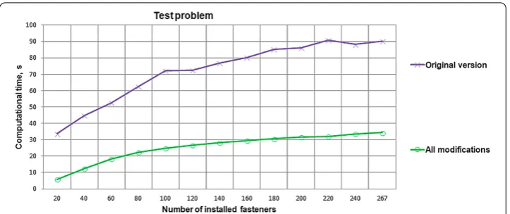
Let us examine how mentioned above modifications of G-I-P algorithm affect the compu-tational speed. We consider test problem with , unknown variables. Let us examine how first three modifications speed up computations. In following plot (see Figure ) the computation time is plotted alongY axis,Xaxis corresponds to number of fasteners in-stalled between joined parts. Violet line corresponds to original algorithm and green line - to the version with all described modifications. It is clearly seen that computation time does increase if more forces are applied to riveted parts, but proposed modifications re-duce the time more than twice in comparison with original version of algorithm.
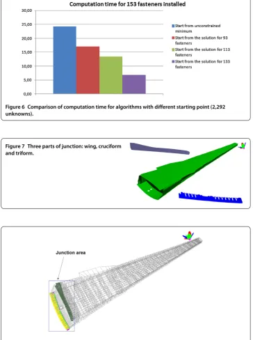
The next bar chart in Figure illustrates the computation time needed to solve test problem if fasteners are installed using modified G-I-P algorithm. We consider several load cases with different initial approximations such as:
• Unconstrained minimum (blue column).
• Solution obtained for fasteners installed (red column). • Solution obtained for fasteners installed (green column). • Solution obtained for fasteners installed (violet column).
Figure 6 Comparison of computation time for algorithms with different starting point (2,292 unknowns).
Figure 7 Three parts of junction: wing, cruciform and triform.
Figure 8 Finite element mesh for wing-to-fuselage assembly.
time from to seconds. This ‘warm start’ technology is quite profitable when making series of computations.
2.3 Applications
.. Wing-to-fuselage assembly simulation
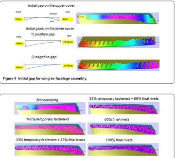
Figure 9 Initial gap for wing-to-fuselage assembly.
Figure 10 Result gap between cruciform and upper wing panel.If area is colored by magenta it means that gap is equal to zero there.
If we examine the finite element mesh of this model we may see that the junction area is quite small in comparison with the whole model (shown by colored dots in Figure ). Thus this model perfectly fits the requirements of proposed methodology.
We are to set the initial gap (see Figure ) and then observe the results when simulating different stages of assembly process.
The resulting gap fields are shown in Figures and . The installed fasteners are shown by yellow dots, final rivets - by blue dots and free holes - by small grey dots.
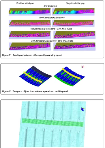
.. Fuselage-to-fuselage assembly simulation
Also we present an example of fuselage-to-fuselage assembly simulation. Let us consider two fuselage panels, as it is shown in Figure .
Figure gives the finite element mesh adjacent to the junction area that is shown by green.
An example of simulation results for this case is given by Figure . Three installed fas-teners are shown by yellow dots and free holes - by small grey dots. In the fasfas-teners’ neigh-borhood the gap is closed (shown by blue color).
Figure 11 Result gap between triform and lower wing panel.
Figure 12 Two parts of junction: reference panel and mobile panel.
Figure 13 Finite element mesh for fuselage-to-fuselage assembly.
3 Conclusions
Developed approach is the most efficient for simulation of aircraft parts’ riveting. The need to perform series of similar computations and a priori known narrow junction area are the main features that allow reducing computational time and resources.
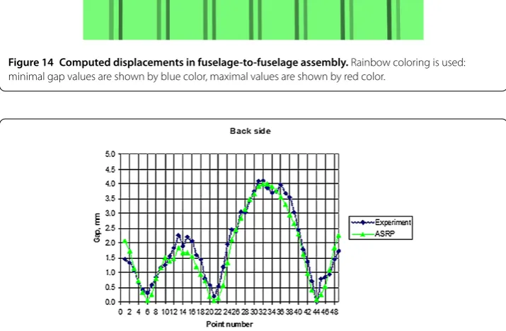
Tech-Figure 14 Computed displacements in fuselage-to-fuselage assembly.Rainbow coloring is used: minimal gap values are shown by blue color, maximal values are shown by red color.
Figure 15 Measured and calculated gaps with three installed fasteners.
nology Readiness Level. TRL means that the technology has passed the thorough testing of prototyping in representative environment. Basic technology elements integrated with reasonably realistic supporting elements. Prototyping implementations conform to target environment and interfaces (see http://esto.nasa.gov/files/trl_definitions.pdf).
Described methodology was fruitfully applied to simulation of real airframe junctions. In particular ASRP complex was successfully tested on airframe junctions for latest Airbus aircraft models like A and A NEO.
Competing interests
Our research was held out as a part of joint project between AIRBUS company and Saint Petersburg State Polytechnic University.
Authors’ contributions
All authors contributed equally to the writing of this paper. All authors read and approved the final manuscript.
Author details
1Department of Applied Mathematics, Saint Petersburg State Polytechnic University, Saint Petersburg, Russian Federation. 2Airbus, Toulouse, France.
Acknowledgements
We would like to thank Jacques Bouriquet, Nicolas Prioul, Claude Gimenez (AIRBUS) and professor Eugene Victorov (Saint Petersburg State Polytechnic University) for their invaluable assistance.
References
1. Lupuleac S, Kovtun M, Rodionova O, Marguet B:Assembly simulation of riveting process.SAE Int J Aerosp2010,
2:193-198.
2. Lupuleac S, Rodionova O, Smirnov A, Shubnikov V, Bretagnol B:Software complex for riveting process simulation.
SAE Technical Paper2011, 2011-01-2772
3. Lupuleac S, Petukhova M, Shinder Y, Bretagnol B:Methodology for solving contact problem during riveting process.SAE Int J Aerosp2011,4:952-957.
4. Pedersen P:A direct analysis of elastic contact using super elements.Comput Mech2006,37:221-231. 5. Wriggers P:Computational Contact Mechanics. 2nd edition. Berlin: Springer; 2006.
6. GoldFarb D, Idnani A:A numerically stable dual method for solving strictly quadratic programs.Math Program
1983,27:1-33.
7. Powell MJD:On the quadratic programming algorithm of Goldfarb and Idnani.Math Program Stud1985,25:46-61. 8. Lupuleac S, Shinder Y, Petukhova M, Yakunin S, Smirnov A, Bondarenko D:Development of numerical methods for
simulation of airframe assembly process.SAE Int J Aerosp2013,6:101-105.
10.1186/2190-5983-4-8