Real-time delay statistics in wireless IP networks

(1)

www.adv-radio-sci.net/10/105/2012/ doi:10.5194/ars-10-105-2012

Radio Science

Real-time delay statistics in wireless IP networks

D. Huo

Bell Laboratories, 67 Whippany Road, Whippany, NJ 07981, USA Correspondence to: D. Huo ([email protected])

Abstract. In the wireless communication, the variation of the transmission delay is called jitter and is one of the vari-ables responsible for the degradation of the service quality. Jitter is present in every section of the transmission system. Its stochastic behavior depends on the technology imple-mented in the system and the service provided by the sys-tem. This paper focuses on mathematical modeling and phe-nomenological analysis of the jitter encountered by the real-time services in a wireless network. Using the data made available to the public by the wireless industry, we explore the stochastic characterizations of the jitter in a wireless IP networks. Within the scope of real-time service, we studied the relation between delay, jitter and the inter-packet time. Evaluation of the sample data indicates a long range de-pendence of the inter-packet time of the received packets in a real-time connection. The result helps understanding the transmission delay encountered by the real-time service over wireless IP networks.

1 Introduction

To provide IP (Internet Protocol) based packet transmission service a wireless network relies on an infrastructure that consists of multiple sections. Each of these sections intro-duces a time delay to the packet transmission. The tempo-rary variation of the time delay is referred to as jitter and it depends not only on the underlying transmission technology, but also on the service the packet transmission is supposed to support. The real-time service requires a fixed transmit and receive rate and, as such, its quality is impaired by the jitter. In wireless technologies such as HSPA (High Speed Packet Data) or LTE (Long Term Evolution), jitter is primar-ily caused by two techniques introduced to improve the radio interface performance: the packet scheduling at the RNC (ra-dio network controller) for UMTS or at the eNodeB for LTE, and the HARQ (hybrid automatic request-response)

(2)

In Sect. 2 we will discuss the definition of the random vari-ables delay and inter-arrival time, and characterize the packet streams of constant rate in a rather general way. Section 3 is dedicated to the characterization of the compound transmis-sion system, consisting of concatenated sub-systems. The mining of the aforementioned data for the purpose of jitter study is performed in Sect. 4, making use of the theory de-veloped in the previous sections. In Sect. 5 we will construct and analyze the mobile-to-mobile connection using existing sample paths, before giving a conclusion in Sect. 6.

2 Transmission system

A packet stream is defined by indexing each packet by a unique integeri∈Z, where Z is the set of integer numbers, so that consecutive packets are packets that should have adja-cent indices. While being transmitted through the transmis-sion system, packet experience delay, which can be deter-mined by measurement at two points: One at the input port of transmission system and the other at the output port of the transmission system. The arrival time, as well as the depar-ture time, is a mapping of the packet index to a real number Z7→R, where R is the set of real numbers. Note that the interpretation of the term “arrival” and “departure” depends on the context, i.e. depending on the system we observe. As far as a pair of transmitter and receiver is concerned, the ar-rival time at the receiver is the time when the packet departs the system of transmission medium that connects the trans-mitter and receiver. For a packet stream with constant data rate, the time between consecutive packets at the data source should be the same. Then,without transmission impairments the arrival time at the receiver is a monotone increasing step function with a fixed increment. Let T (i)denote the time when the packet with indexi departs the transmitter. Then T (i)=C+i/rfori∈Z, where the real numberr >0 is the packet rate andCis the reference time. It is reasonable to as-sume that all packets in a packet stream are generated in or-der at the transmitter, i.e.T (i) < T (j )for i < j. Lett (i)be the time when the same packet arrives at the receiver. Then, t (i) > T (i)for alli∈Z. Obviously, the transmission delay of a packetd(i)=t (i)−T (i)is positive for any non-trivial transmission system. Moreover it in fact a random number. For the further study, we make the assumption that the de-lay is a random variable defined in(,B,P), whereis the space of random event, B the Borel algebra on real numbers and P the probability measure. Sincet (i)=C1+d(i)+i/r

withC1 accounting for the fixed delay of the system and

the reference time at the transmitter, it is readily seen that t (i)−E{t (i)} =d(i)−E{d(i)}, whereE{}refers to the sta-tistical expectation.

Another related random number is the inter-packet time. As mentioned before, with the term of inter-packet time we could be talking about the arrival time or the inter-departure time, depending on the context. For both cases the

Table 1. Example of re-ordering.

i 0 1 2 3 4 5 ...

t (i) 10 11 14 12 13 15 ...

π◦t (i) 10 11 14 14 14 15 ...

inter-packet time is a mapping of indexx:Z7→R. In partic-ular, the inter-arrival time at the receiver is well defined by x(i)=t (i)−t (i−1)for limi→−∞t (i)=0, and we have

Proposition 1 Between the inter-packet time and the delay there are following relations

x(i)=d(i)−d(i−1)+1

r (1)

d(i)=d(0)+ i

X

k=0

x(k) (2)

For a stable transmission system, we can assume the sta-tionarity. Then E{d(i)} =E{d(i−1)}andE{x(i)} =1/r, meaning the transmission system does not change the aver-age inter-packet time, which is a necessary requirement of the real time service. Assuming the packet loss is handled by the upper layer protocol, we can ignore the packet loss in our study. Normally a packet with smaller index will arrive ear-lier that one with a larger index. But, due to the randomness of the delay, a packet with smaller index may be received later than a packet with larger index, resulting in packet dis-order in the packet stream at the receiver. The requirement of order preservation for the delivery of real-time services ne-cessitates a posterior re-ordering operation at the receiver: It is a mapping of a set of the packet indices into itself, so that the sequential order of the packets is restored as given by the source. While the re-ordering action re-shuffles the received packets for the purpose of re-establishing the original order, it modifies the receive time, resulting in jitter.

Definition 1 Let Z be the set of all packet indices and R the set of the departure time. A re-ordering operation is a map-pingπ:Z×R7→Z×R and fori < j

π(i,t ):=(π◦t )(i)=

t (j ), for t (i) > t (j )

t (i), for t (i)≤t (j ) (3) The operationπ permutes the packets with respect to the in-dices. Thus, for a given positiveτ∈R,

(3)

Generally speaking the re-ordering introduces delay: Proposition 2 Lett (i)be the departure time of packetiand V ar{t (i)}<∞. Then, for the re-ordering functionπ:Z× R7→Z×R, there is(π◦t )(i)≥t (i)

Proof: The re-ordering operation works index after index in ascending order, starting from a pointi=0. Ift (i)≥t (i− 1), then the order between packetiand packeti−1 is not changed by the transmission system, hence there is no need of re-ordering and(π◦t )(i)=t (i). But, ift (i) < t (i−1), then a disorder occurs during the transmission, there is a need of re-ordering which mapst (i)to a number no less thant (i− 1), resulting in(π◦t )(i) > t (i). QED. How does the re-ordering affect the inter-arrival time and jitter ? Using the knowledge obtained so far, we can draw the following conclusion for the inter-arrival time: For x(i)≥ 0, no ordering is needed, as there is no disorder. A re-ordering operation due whenx(i) <0 is . Starting fromi, one checks throughj=i,i+1,..,i+m−1 untili+mwithx(i+ m)≥0. Then, all those packets need to be buffered because they are out of order. Hence, the re-ordering operation is equivalent to setting(π◦x)(j ):=0 forj∈ [i,i+m−1]and (π◦x)(i+m):=x(i+m)−Pi+m−1

j=i x(j ). Then, it follows

i+m

X

j=i

(π◦x)(j )=x(i+m)− i+m−1

X

j=i

x(j ) (5)

Now, assume that the arrival afteri+m−1 is ordered forn > 0 consecutive packets, i.e.x(j )≥0 withj∈ [i+m,i+m+n] until againx(i+m+n+1) <0. Then

i+m+n

X

j=i+m

(π◦x)(j )= i+m+n

X

j=i+m

x(j ) (6)

Thus, we obtain finally i+m+n

X

j=i

(π◦x)(j )= i+m+n

X

j=i+m x(j )−

i+m−1

X

j=i

x(j )≥ i+m+n

X

j=i

x(j )(7)

meaning that the inter-arrival time tends to increase after the re-ordering operation at the receiver. The conclusion can be formalized as the following

Corollary 1 lim n→∞P r{

1 n

n

X

i=1

[(π◦x)(i)−x(i)] ≥0} =1

Proof:: Consider the set N = {1,2,....,n} of n elements andN =N+∪N− with N+∩N−= ∅, where N+= {i∈ N|x(i)≥0}andN−= {i∈N|x(i) <0}. Then

X

j∈N+

[(π◦x)(j )−x(j )] =0 (8)

and

X

j∈N−

[(π◦x)(j )−x(j )]>− X j∈N−

x(j )≥0 (9)

where the equal sign applies whenN−= ∅. Hence E{1

n

X

j∈N

[(π◦x)(j )−x(j )]} ≥0 (10)

Since the process is stationary, the relation holds forn→ ∞

and the weak convergence follows. QED

3 Compound transmission system

A heterogeneous transmission path can be decomposed into mutual independent sections. We call such a transmission system a compound system, consisting of concatenated sub-systems. In the chain of concatenated sub-systems the packet departure time at one sub-system is at the same time the packet arrival-time for the following sub-system. Thus, the delay observed at the output of the very last sub-system in the chain is the accumulation of delays from all sub-systems. Let dk(i)denote the packet delay caused by thek-th sub-system andxk(i)the corresponding inter-packet time. Denoting the random delay of thei-th packet of the compound system ofn sub-systems withDn(i), we haveDn(i)=Pn

k=1dk(i).

Ac-cordingly, the inter-packet timeXn(i)of thei-th packet of the compound system can be determined by

Xn(i)=Dn(i)−Dn(i−1)+ 1 Rn

(11) following the equation (1). Then,

E{Xn− 1 Rn} =

n

X

k=1

E{xk− 1

rk} (12)

Therefore, we have the following result:

Proposition 3 For a compound system of n independent concatenated sub-systems,

E{Xn} = 1

Rn (13)

whenE{xk} =1/rk for k=1,2,...,n. Then, the variances are subject to

V ar{Xn} = n

X

k=1

V ar{xk}. (14)

The second statement follows from the independence be-tween the sub-systems, i.e.E{(xk−1/rk)(xi−1/ri)} =0 for k6=i, and it indicates a spreading of the variance as result of concatenation. Moreover, ifE{dk(i)−dk(i−1)} =0 for all i∈Z andk=1,..,n, we haveRn=rk=r.

(4)

At each inter-face between the sub-systems, the inter-packet time can be positive or negative. Negative inter-packet time means packet index disorder in the packet stream. The inter-packet time after the re-ordering operation is always non-negative.

4 Data mining 4.1 Radio interfaces

All modern wireless networks utilize the techniques of re-source sharing over the air-interface. Users are multiplexed onto the frequency and time resources, using radio tech-nologies such as CDMA (Code Division Multiple Access), TDMA (Time Division Multiple Access), OFDMA (Orthog-onal Frequency Division Multiple Access) or any combina-tion of them, to achieve spectrum efficiency and thus the net-work capacity. The radio-interface HSPA is based on CDMA with dynamic resource allocation. Similar to LTE, the pro-tocol architecture of HSPA consists of, from bottom to top, PHY(Physical Layer) –MAC(Medium Access Control Pro-tocol) – RLC(Radio Link Control ProPro-tocol) –PDCP(Packet Data Convergence Protocol) – IP(Internet Protocol), from bottom to top, with services carried in the payload of IP stack. A critical entity in the MAC layer is the HARQ that combines the request-response protocol and the adap-tive channel coding to enhance the link performance. While improving the throughput of the radio channel, HARQ also introduces packet delay that varies with the changing radio channel condition. The merit is similar to that of a scheduler implemented at the radio network controller to assign radio resource among users and services, so that the air-interface can be fairly shared and the resource utilization be optimized. While scheduler and HARQ are essential for the performance of the radio interface, both introduce delay variation. Thus, through HARQ and the scheduler, the delay performance of a wireless network depends on both the radio channel condi-tion and the cell traffic demand. As result, the jitter occurs. A project of 3GPP-RAN1 (2011) has provided ample simula-tion data for HSPA air interface performance in 3GPP-RAN1 (2006), in which traces of the packet delay and packet loss are recorded. Following 3GPP-SA4 (2006), the data were produced for the purpose of development of voice codec. As such, they are ideal for the study of the jitter behavior in an wireless cellular environment, because the underlying net-work configuration, channel conditions and traffic loads are predetermined and normalized by the standard development organizations, and as such are representative and authentic. We will make use of those data in the sequel.

4.2 Stochastic sample paths

In 3GPP-RAN1 (2006), an input stream of identical packets was sent every 20 ms, and the packet delay and packet loss at the receiver were recorded for each packet. The samples

Table 2. Slope of the regression line as a two dimensional distribu-tion.

j = ACF PER VAR

a(j,i) = −α(ACF,i) −β(PER,i) −γ (VAR,i)

for the down-link (DL) are collected on the RLC layer at the mobiles with a fixed geometry, while the samples for the up-link (UL) are collected on the RLC layer at RNC. The cellular network consists of 19 cells, each with 3 sectors. The 4 channel models used are based on ITU-R (2012):

– Pedestrian A with 3 km h−1(PA3), – Pedestrian B with 3 km h−1(PB3), – Vehicular A with 30 km h−1(VA30), – Vehicular A with 120 km h−1_(VA120),

representing the different speed of mobility with respective channel model. In addition, 4 intensities of traffic load are considered:

– 40 users per sector (40U), – 45 users per sector (45U), – 60 users per sector (60U), – 100 users per sector (100U).

(5)

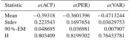
Table 3. Slope statistic for the DL (df=35).

Statistic a(ACF) a(PER) a(VAR) Mean −0.39318 −0.3601396 −0.4713244 Stdev 0.223543 0.1697654 0.03629753 90 %-EM 0.048695 0.036981 0.007907

H 0.803409 0.8199302 0.76433781

Definition 2 A stochastic processX(t )is self-similar when it has a distribution identical to that ofw−HX(wt )fort >0, w >0 and 0.5< H <1, whereH is called the Hurst param-eter andwthe scaling factor. A stationary stochastic process is called a fractional Brownian motion when

1. X(0)=0

2. X(t2)−X(t1)has a Gaussian distribution fort1< t2

3. E{X(t2)−X(t1)} =0

4. Var{X(t2)−X(t1)} ∝ |t2−t1|H for 1/2< H <1

Based on this definition, long range dependence of stochastic process can be quantified by the Hurst parameter H, which can be estimated by means of proper asymptotes, as we will do in the following.

4.3 Asymptotes

For the packet inter-arrival time, the following second-order statistics can be computed using the sample paths:

1. Autocorrelation(ACF) :

ρ(k)=Cov{x(· +k)x(·)}

Var{x(·)} (15)

fork∈Z withρ(k)=O(k−α)for k→ ∞. 2. Periodogram(PER):

p(ω)= 1 2π n|

n

X

k=1

[x(k)−E{x}]ekω

√

−1_|2 ₍₁₆₎

for sufficiently largen >1 with p(ω)=O(ω−β)forω→0. 3. Variance (VAR):

σ2(k)=Var{1 k

k

X

i=1

x(i)} (17)

for largek >1 withσ2(k)=O(k−γ)for k→ ∞.

Table 4. Slope statistic for the UL (df=17).

Statistic a(ACF) a(PER) a(VAR) Mean −0.36799 −0.2607483 −0.4728221 Stdev 0.162307 0.2737584 0.02107574 90 %-EM 0.050881 0.085819 0.006607

H 0.816006 0.6303742 0.76358897

In the above asymptotes, the speed of the decay character-izes the dependence between entries in the sample path. A stochastic process is self-similar, when the sample estimate ofρ(k)andσ2(k)tends tok−α for large sample sizekand α >1/2, or equivalently the sample estimate ofp(ω)tends to ω−β for 1< β <2 for smallω. The Hurst parameterHused to characterize the self-similar process is related to the power of the asymptotes throughH=1+α/2=(1+β)/2. The stochastic process has the long range dependence when the corresponding Hurst parameter is in the range of 0.5< H < 1. In order to obtain an estimation of this parameter from our samples, we observe the slope of logarithm of the respec-tive second order statistics, i.e. the parametera(ACR,i)=α, a(PER,i)=β, a(VAR,i)=γ, respectively. In more gen-eral term, as shown in Table 2, we observe the two dimen-sional variables a(j,i), wherej is the category index with j=ACR,PER,VAR, andi is the index of the sample path used.

Using all 54 samples, the intercept and the slope of the log-arithm of the autocorrelation, the periodogram and the vari-ance are estimated, respectively: All in total, 36 slopes are estimated for the down-link, while 18 slopes are estimated for the up-link. The sample mean of the slope a(ACF,i), a(PER,i)anda(VAR,i)are computed by averaging overi, resulting in

a(ACF)= 1 ns

ns

X

i=1

a(ACF,i),

a(PER)= 1 ns

ns

X

i=1

a(PER,i),

a(VAR)= 1 ns

ns

X

i=1

a(VAR,i),

wherens is the number of samples. The results are shown in Tables 3 and 4 for the down-link and the up-link, respec-tively. The 90 percent confidence interval is also computed for Student-t distribution and shown as the error margin, i.e. 90 %-EM in the tables.

(6)

Table 5. Estimated H.

Hurst

Link Parameter Stdev. #Samples

DL 0.796 5.26 86×3=258

UL 0.747 1.20 18×3=54

5 Mobile-to-mobile connection

A mobile-to-mobile connection requires at least an up-link, a down-link and at least an intermediate node representing the core network. However, since we only have sample paths for the radio interface, it is reasonable to focus our atten-tion to the jitters caused by the air-interface on the jitter. For this purpose, the model can be simplified by assuming that the core network processes the incoming traffic accord-ing to a deterministic round-robin scheduler. As result, the observed statistics of the mobile traffic will not be affected by the other traffics that join the node in the core network, which adds only a fixed delay to the packet stream of the refrence mobile traffic. Thus, the inter-arrival time, hence the jitter, becomes independent of the core network under this assumption, and we are left with a concatenation of only two sub-systems: One is the up-link radio interface and the other is the down-link radio interface. Using data available in 3GPP-RAN1 (2006) for up-link and down-link, one can construct new sample paths to study the jitter statistics of an end-to-end connection. Now that the compound system con-sists of two concatenated sub-systems, 4 groups of new sam-ple paths can be generated, by combining four different types of sub-systems, i.e. low mobility (lm), high mobility (hm), low traffic (lt), high traffic (ht). The existing sample paths can, according to their respective physical configuration, be associated with these 4 groups as the following,

1. lm-lt: low mobility and low traffic (PA3,PB3,VA30; 40U)

2. hm-lt: high mobility and low traffic (VA120; 40U) 3. lm-ht: low mobility and high traffic (PA3, PB3,VA30;

100U)

4. hm-ht: high mobility and high traffic (VA120; 100U) for the down-link and as

1. up-lm: low mobility (PA3,PB3,VA30) 2. up-hm: high mobility(VA120)

for the up-link. Since the inter-packet time of the sub-systems demonstrates long range dependence, we are inter-ested in the same long range dependence of the inter-packet time in a compound system. To find more about this, let ρ(k)denote the autocorrelation function of the inter-packet

Table 6. Estimatedαcof the mobile-to-mobile connections.

Mean Stdev 90 % EM

0.078454 0.369239 0.027325

time of the compound system, andρi(k)be the autocorrela-tion funcautocorrela-tion of the inter-packet time of the sub-systems with i=1,2,...m. When independence among the sub-systems is assumed, we have

ρ(k)= m

X

i=1

ρi(k)wi (18)

for anyk≥0, where wi=

Var(xi)

Pm

i=1Var(xi)

(19) By arranging the terms on the right hand in ascending order of magnitudeαi,

lim k→∞ρ(k)

= m

X

i=1

lim

k→∞ρi(k)wi

=k−αc_(w

1c1+

w2c2k−α2+αc+...+wmcmk−αm+αc)

forαc=min1≤i≤mαiandci>0 withi=1,2,..m. This indi-cates that the asymptote of the auto-correlation is dominated by the sub-system with the slowest decay. As an example we evaluate the parameter of the concatenated system consisting of 18 up-link samples and 18 down-link samples, randomly selected from the available data base. Combining them to make an end-to-end connection results in 18×18=324 sam-ples. Now parameterαc is estimated using these 324 sam-ples, the result is shown in Table 6. Comparing to the num-bers in Table 3 and 4, the estimatedαcin Table 6 is less than bothα0 andα1. Thus, the example is consistent with the

analysis. On the other hand, when the constantsci are also taken into account, we obtain the following more accurate result:

Proposition 4 For a compound system of m concatenated independent sub-systems, assume the processes of inter-departure timexiare pair-wise independent fori=1,2,..,m, and the autocorrelation functionρi(k)for thei-th subsystem has the asymptotic limk→∞ρi(k)=cik−αi with ci>0 and

αi>0. Then, the autocorrelation function of the compound systemρ(k)has the asymptotic behavior

lim k→∞ρ(k)

=O(k−αc₎ ₍₂₀₎

with αc≤

Pm i=1αiciwi

Pm

i=1ciwi

(7)

Proof: Introducingcw=Pm

i=1ciwi in (18) we obtain

lim k→∞ρ(k)

=cw m

X

i=1

k−αi_ci_wi_/cw ₍₂₂₎

The sum on the right hand of the equation can be viewed as the expectation of the convex functionk−u. By Jensen’s inequality,

k−mini≤i≤m(αi)_≥

m

X

i=1

k−αiciwi

cw ≥k

−Pm

i=1αici wi_cw ₍₂₃₎

forcw>0 andαi>0. Since ln(k−u₎_≥_ln(k−v₎_for_u_≤_v, lim

k→∞

−ln[ρ(k)] ln[k] ≤

m

X

i=1

αiciwi cw

(24)

Obviously, the term on the left hand isαcand the equal sign holds whenαc=αifori=1,2,...,m. QED.

6 Conclusions

So far we have studied the jitter statistics experienced by the real time service like voice, when packet streams are trans-mitted over HSPA wireless systems, using analytical as well as empirical methods. By analysis we established the rela-tionship between delay and inter-packet time, and investi-gated the stochastic behavior of those quantities. With help of simulation data available for HSPA, we could estimate the second order statistics of the jitter and evaluate their asymptotes. Combining the existing samples to construct new samples representing new physical scenarios allows us further to investigate the jitter statistics of a mobile-to-mobile connection.

An important assumption made here was that the service provided by the packet stream requires rate preservation, i.e. the data are generated with constant rate and also expected to be received with the same rate. This requirement makes it necessary to deploy buffer to enable ordering at the re-ceiving end. Only the operation of re-ordering can mitigate the delay jitter introduced by the deployment of the scheduler and the HARQ in a wireless transmission system. Evaluation of the sample paths with respect to the asymptotic decay of the autocorrelation, the periodogram and the variance reveals a statistical long range dependence of the inter-packet time, where the power law of the asymptote of the orderk−α has typically 1/2< α <1. For a compound system consisting of concatenated sub-systems, the long range dependence behav-ior of the compound system is dominated by the sub-system with the slowest decay, a finding confirmed by the sample evaluation.

References

3GPP(Third Generation Partnership Project): “TS 36.300 V8.8.0”, available at: http://www.3gpp.org, Aug. 2012.

3GPP: “LS on RAB and the error-delay-profile for the performance characterization of VoIMS over HS-DPA/EULLS”, RAN1-44, 13–17 Febuary 2006, Denver, avilable at: http://www.quintillion.co.jp/3GPP/TSG RAN/ TSG RAN2006/TSG RAN WG1 RL1 2.html, Aug. 2012. 3GPP, “Specification 25 Series”, RAN1, available at: http://www.

3gpp.org July, 2011.

3GPP: “Working Document for the Performance Characteriza-tion of VoIMS over HSDPA/EDCH, v0.0.4”, 3GPP-SA4-40, 28 August–2 September 2006, Sophia-Antipolis, available at: http://www.3gpp.org, Dec. 2006.

International Telecommunications Union, “Guidelines for Evalua-tion of Radio Transmission”, RecommendaEvalua-tion ITU-R M.1225, available at: http://www.itu.int/rec/R-REC-M.1225/en, April, 2012.

Paxson, V.: “Fast Approximation of Self-Similar Network Traffic”, LBL-36750, Lawrence Berkeley Laboratory, April, 1995. Geist, R. and Westall, J.: “Practical Aspects of Simulating Systems

Having Arrival Processes with Long-range Dependence”, IEEE Proc. of the 2000 Winter Simulation Conference, 2000. Mandelbrot, B. B.: Mutifractals and 1/f Noise, Springer-Verlag,

1998.

Beran, J.: Statistics for Long-Memory Processes, Chapman and Hall, 1994.

Crovella, M. E. and Bestavros, A.: Self-Similarity in World Wide Web Traffic: Evidence and Possible Causes, IEEE/ACM, Trans. on Networking, 5(6), December, 1997.

Taqqu, M., Willinger, W., and Sherman, R.: Proof of a Fundamen-tal Results in Self-Similar Traffic Modeling, ACM SiGCOMM Compiuter Communication Review, 27(2), 5–23, April, 1997. Willinger, W., Taqqu, M. S., Sherman, R., and Wilson, D. V.:

Self-Similar Through High-Variability: Statistical Analysis of Eth-ernet LAN Traffic at the Source Level, IEEE/ACM, Trans. on Networking, 5(1), February, 1997.

Willinger, W., Taqqu, M. S., Sherman, R., and Wilson, D. V.: On the Self-Similar Nature of Ethernet Traffic (Extended Version), IEEE/ACM Trans. on Networking. 2(1), 1–15, February, 1994. Park, K. and Willinger, W. (Ed.): Self-Similar Network Traffic and