The Thirty-Third AAAI Conference on Artificial Intelligence (AAAI-19)
Primarily about Primaries
Allan Borodin
University of TorontoOmer Lev
Ben-Gurion UniversityNisarg Shah
University of Toronto [email protected]Tyrone Strangway
University of Toronto [email protected]Abstract
Much of the social choice literature examinesdirectvoting systems, in which voters submit their ranked preferences over candidates and a voting rule picks a winner. Real-world elec-tions and decision-making processes are often more complex and involve multiple stages. For instance, one popular voting system filters candidates throughprimaries: first, voters affil-iated with each political party vote over candidates of their own party and the voting rule picks a candidate from each party, which then compete in a general election.
We present a model to analyze such multi-stage elections, and conduct the first quantitative comparison (to the best of our knowledge) of the direct and primary voting systems with two political parties in terms of the quality of the elected candi-date. Our main result is that every voting rule is guaranteed to perform almost as well (i.e., within a constant factor) under the primary system as under the direct system. Surprisingly, the converse does not hold: we show settings in which there exist voting rules that perform significantly better under the primary system than under the direct system.
Introduction
If I could not go to heaven but with a party, I would not go there at all.
– Thomas Jefferson, 1789
Thomas Jefferson, like many of the US constitution’s au-thors, believed that political parties and factions are a bad thing (see also Hamilton, Madison, and Jay (1787)). This view stemmed from a long history of British and English political history, in which prison sentences and executions were possible outcomes in the battle between factions for supremacy at the Royal court (Simms 2007). However, both in Britain and in the Unites States, once their respective leg-islative assemblies gained political force, parties turned out to be quite unavoidable. Even Jefferson had to start his own party, which ended up quite successful, and was able to van-quish the opposing party from political existence (Wilentz 2005).
Fast forwarding to today, political parties have become the bedrock of parliamentary politics throughout the world. In particular, one of political parties’ main roles – if not the
Copyright c2019, Association for the Advancement of Artificial Intelligence (www.aaai.org). All rights reserved.
most important (especially in presidential systems) – is to se-lect the candidates which are voted for by the general public. The mechanisms by which parties make this selection are varied, and they have evolved significantly throughout the past 150 years. But in the past few decades there has been a marked shift by parties throughout the world towards in-creasing the ability of individual party (or unaffiliated) mem-bers to influence the outcome, and in some cases, to be the only element to determine party candidates (Cross and Blais 2011). In particular, US parties have changed their election methods since the 1970s to focus the selection of presiden-tial, congressional and state-wide candidates on popular sup-port by party members via primaries (Cohen et al. 2008).
Despite this long and established role of parties in whit-tling down the candidate field in elections, the treatment of a parties’ role in elections within the multiagent systems community has been quite limited. While various candidate manipulation attacks have been investigated (e.g., Sybil at-tacks (Conitzer and Yokoo 2010)), and there is recent re-search into parties as a collection of similar minded candi-dates (e.g., in gerrymandering, across different districts), the role of parties in removing candidates has not been explored. The focus of this paper is theprimaryvoting system, in which each party’s electorate selects a winner from among the party’s candidates, and among these primary winners, an ultimate election winner is selected by the general public. Our goal is to compare this system to thedirectvoting sys-tem, in which all voters directly vote over all candidates.
Our Results
Our contribution is twofold. First, we formulate a model which allows a quantitative comparison of the two voting systems. Our model is a spatial model of voting in which voters and candidates lie in an underlying multi-dimensional space, and voter preferences are single-peaked. This allows us to compare each candidate’s social utility in terms of its total distance to the voters. We make the evaluation met-ric formal using the notion of distortion advocated by a recent line of research (Procaccia and Rosenschein 2006; Boutilier et al. 2015). Our results focus on 2 parties, each selecting a single candidate, with both candidates presented to the general voting public.
that no voting rule performs much worse (by more than a constant factor) under the primary system than under the direct system. While the converse holds in some cases, we show settings in which it does not, and there exist voting rules that perform much better under the primary system than under the direct system.
It is important to note that while we write of parties, vot-ers and elections, this multi-step model applies to a vari-ety of decision-making processes by agents. An organiza-tion selecting an “employee of the month” may ask each unit to nominate a single candidate, and then choose from amongst them. A city may ask its regional subdivisions to assess which roads require urgent fixing, and then the city council decides from these options where to invest its efforts. Fundamentally, in many cases where the potential number of options is huge, it is common to use subdivisions to cull the options and present only a few of them for discussion and vote. In such cases, our multi-stage model is apt.
Related Work
The analysis of regular, direct elections is long and varied, both in the social sciences and in AI (Brandt et al. 2016). In our particular setting, the voters are located in a metric space, with their preferences related to their distance from candidates. Such settings have been widely investigated in the social science literature since the work of Downs (1957), recently summarized by Schofield (2008). In particular, we focus on the idea of distortion in such elections, a topic broached by Procaccia and Rosenschein (2006) for voters with a utility function, but investigated in the context of voters in metric spaces in a series of papers (Anshelevich, Bhardwaj, and Postl 2015; Anshelevich and Postl 2017; Skowron and Elkind 2017) for most common voting rules. Feldman, Fiat, and Golomb (2016) explored such a setting for strategyproof mechanisms.
Discussing changes to the set of candidates has been mainly focused on two paths of research. Strategic candi-dates, investigation of which began with the work of Dutta, Jackson, and Le Breton (2001) – followed by Dutta, Jack-son, and Le Breton (2002) discussing strategic candidacy in tournaments, and recently further explored by Brill and Conitzer (2015), Polukarov et al. (2015) and others – deals mainly with finding equilibria. The other is the addition and removal of candidates, as a form of control manipulation, which was studied by Bartholdi III, Tovey, and Trick (1992); see the summaries by Brandt et al. (2016) and Rothe (2015). Investigating parties’ selection methods and their effect on the election has mostly been done in the social sciences. Kenig (2009) details the range of selection methods parties use, and there has been significant focus on more demo-cratic methods for leader selection (Cross and Katz 2013), which seems to be a general trend in many Western coun-tries (Cross and Blais 2011). There is also significant lit-erature on particular party elections in various countries, such as Britain (Jobson and Wickham-Jones 2010), Belgium (Wauters 2010), Israel (Hazan 1997), and many others. Nat-urally, the most widely examined country is the US, in which political parties have been a fixture of political life since its
early days (Wilentz 2005). The most recent extensive sum-mary of research on it is due to Cohen et al. (2008), who try to explain how party power-brokers influence the party membership vote. Norpoth (2004) uses primary data to pre-dict election results, and notably Sides et al. (2018) show that primary voters are very similar to “regular” voters. In computational fields, recent interest in proxy voting (Cohen-sius et al. 2017; Kahng, Mackenzie, and Procaccia 2018), in which voters give other agents the ability to vote for them, may be related to how modern parties are viewed and ana-lyzed.
Model
For k ∈ N, define [k] = {1, . . . , k}. Let V = [n]
de-note a set ofnvoters, andAdenote a set ofmcandidates. We assume that voters and candidates lie in an underlying metric space M = (S, d), whereS is a set of points and
d is a distance function satisfying the triangle inequality and symmetry. More precisely, there exists an embedding
ρ:V ∪A→Smapping each voter and candidate to a point inS. For a setX ⊆V ∪A, we slightly abuse the notation and letρ(X) = {ρ(x) :x∈X}. Also, forx, x0 ∈V ∪A, we often used(x, x0)instead ofd(ρ(x), ρ(x0))for notational convenience.
In this work, we assume that voters and candidates addi-tionally have an affiliation with a political party. Specifically, we study a setting with two parties1, denoted−1and1. The
party affiliationfunctionπ :V ∪A→ {−1,1}maps each voter and candidate to the party they are affiliated with. For
p ∈ {−1,1}, let Vp = π−1(p)∩V,Ap = π−1(p)∩A,
np = |Vp|, andmp = |Ap|. We requirenp ≥ 1 for each
p ∈ {−1,1}. Our main result (Theorem 2) holds even if there are independent voters not affiliated with either party.
Collectively, aninstanceis the tupleI= (V, A, M, ρ, π). GivenI, our goal is to find a candidatea ∈Aas the win-ner. The social costof ais its total distance to the voters, denotedCI(a) =P
i∈V d(i, a). For partyp∈ {−1,1}, let
CI p(a) =
P
i∈Vpd(i, a). HenceC
I(a) =CI
−1(a) +C1I(a). We also use for X ⊆ V,CXI(a) = P
i∈Xd(i, a). Given
an instanceI, we would like to choose a candidateaOPT ∈ arg mina∈ACI(a)that minimizes the social cost. We shall
drop the instance from superscripts if it is clear from the context.
However, we do not observe the full instance. Specifically, we do not know the underlying metricM or the embedding functionρ. Instead, each voteri∈Nsubmits a avote, which is a ranking (strict total order)iover the candidates inA
by their distance to the voter. Specifically, for all i ∈ N
anda, b ∈ A,a i b ⇒ d(i, a) ≤ d(i, b). The voter is
allowed to break ties between equidistant candidates arbi-trarily. The vote profile−→I = (1, . . . ,
n)is the
collec-tion of votes. Given an instanceI, its correspondingelection
EI = (V, A,−→I, π)contains all observable information.
In the families of instances that we consider, we fix the
1
number of candidatesmand let the number of votersnto be arbitrarily large. This choice is justified because in many typical elections (e.g., political ones), voters significantly outnumber candidates. LetIα
m,Mbe the family of instances
satisfying the following conditions.
• Each party has at least anαfraction of the voters affiliated with it, i.e.,np ≥α·nfor eachp∈ {−1,1}. Note that
α∈ [0,0.5]:α= 0.5is the strictest (exactly half of the voters are affiliated with each party), whileα= 0imposes no conditions; in the latter case, we omit the superscript
α.
• The number of candidates is at mostm.
In particular, we shall focus on a few cases ofM:
M=? This allowsMto be an arbitrary metric space. M=Rk The metric space should beM = (
Rk, d), where
dis the standard Euclidean distance.
M=sep-Rk This means the embedding ρ must be such
thatρ(V−1∪A−1)andρ(V1∪A1)are linearly separable.2 In this case we shall take the metric to beM = (Rk, d)
withdas the standard Euclidean distance. In plain words, the voters and candidates affiliated with each party reside in a certain part of the metric space, separate from those affiliated with the other party. In a single dimension, this means there exists a threshold on the line such that voters and candidates affiliated with one party lie to the left of it, while those affiliated with the other party lie to the right. Note that this is the only choice ofMthat restricts the embeddingρbased on party affiliationπ.
These families of instances are related by the following relation. For allk,
Iα m,sep-Rk
⊂ ⊂
Iα
m,Rk
Iα m,sep-Rk+1
⊂
⊂ I
α
m,Rk+1 ⊂ Im,?α
Voting Rules and Distortion
A voting ruleftakes an election as input, and returns a win-ning candidate fromA. We say that the cost-approximation off on instanceIis
φ(f, I) = C
I(f(EI))
mina∈ACI(a)
,
and given a family of instancesI, the distortion off with respect toIis
φI(f) = sup
I∈I
φ(f, I).
Since distortion is a worst-case notion, we have that when I ⊆ I0,φI(f)≤φ
I0(f)for every voting rulef.
Standard voting rules choose the winning candidate in-dependently of party affiliations. These include rules such as plurality, Borda count, k-approval, veto, and STV. We refer readers to the book by Brandt et al. (2016) for their
2
Two sets of points are linearly separable if the interiors of their convex hulls are disjoint, or equivalently, if there exists a hyper-plane that contains each set in a distinct closed halfspace.
definitions. We call a voting rule affiliation-independent
if f(E) = f(E0) when elections E and E0 differ only in their party affiliation functions. Since an affiliation-independent voting rulefignores party affiliations, we have
φIα m,sep-Rk
(f) = φIα
m,Rk
(f). All of the above-mentioned
rules, in addition to being affiliation-independent, share the property of being unanimous, i.e., they return candidatea
whenais the top choice of all voters.
Stages and Primaries
Given an affiliation-independent voting rulef, voting sys-tems with primaries employ a specific process to choose the winner, essentially resulting in a different voting rulefbthat operates on a given electionE= (V, A,−→, π)as follows:
1. First, it creates twoprimary elections: forp ∈ {−1,1}, define Ep = (Vp, Ap,
− →
p, πp), where
− →
p denotes the
preferences of voters in Vp over candidates in Ap, and
πp:Vp→ {p}is a constant function.
2. Next, it computes the winning candidate in each primary election (primary winner) using rulef: forp∈ {−1,1}, leta∗p=f(Ep).
3. Finally, letEg = (V,a∗−1, a∗1 , − →
g, π)be the general
election, where−→g denotes the preferences of all voters
over the two primary winners. The winning candidate is
b
f(E) = maj(Eg), which is what most voting rules
be-come when dealing with only 2 candidates.3Here, maj is the majority rule, which, given two candidates, picks the one that a majority of voters prefer; our results are inde-pendent of its tie-breaking.
This resembles systems employed by the main US, Cana-dian and other countries’ parties, in which a party’s mem-bers vote on their party’s candidates to select a winner of their primary. In other systems, such selection could be a multi-stage process.
Given an affiliation-independent voting rule f, the goal of this paper is to compare its performance under thedirect system, in whichf is applied on the given election directly, to its performance under theprimary system, in whichfbis applied on the given election instead. Formally, given a fam-ily of instancesIand an affiliation-independent voting rule
f, we wish to compare φI(f) andφI(fb)(henceforth, the distortion of f with respect to I under the direct and the primary systems, respectively).
Small Primaries Are Terrible
Recall that in a family of instancesIαm,M, we require that
at leastαfraction of voters be affiliated with each party, i.e.,
np≥αnfor eachp∈ {−1,1}. In other words, each primary
election must have at leastαnvoters.
3
We first show that when a primary election can have very few voters (α= 0), every reasonable voting rule has an un-bounded distortion in the primary system, even with respect to our most stringent family of instancesIm,sep-R.
Theorem 1. For m ≥ 3, φIm,sep-R(fb) = ∞ for every
affiliation-independent unanimous voting rulef.
Proof. Consider an instanceI∈ Im,sep-Rin which voter1is
located at0and affiliated with party−1, while the remaining
n−1voters are located at1and affiliated with party1. All
mcandidates are affiliated with party−1: one is at0, and the rest are at1.
The candidate a∗ at 0 becomes the primary winner of party−1, and trivially becomes the overall winner. Its so-cial cost is C(a∗) = n−1. In contrast, an optimal can-didateaOP T at 1 has social costC(aOP T) = 1. Hence,
C(a∗)
C(aOP T) = n−1. Since the number of voters n is
un-bounded,φIm,sep-R(fb) =∞.
Theorem 1 continues to hold even if we require that at least a constant fraction of candidates be affiliated with each party: we could simply move a constant fraction of the can-didates from1to3, and the proof would still go through.
On the other hand, if we require that at least aconstant fraction of voters be affiliated with each party, the result changes dramatically.
Large Primaries Are Never Much Worse
For every affiliation-independent voting rule f, we bound the distortion offbin terms of the distortion off for every instance. Note that this is stronger than comparing the worst-case distortions off andfbover a family of instances.Given an instance I = (V, A, M, ρ, π) and party p ∈ {−1,1}, we say that Ip = (Vp, Ap, M, ρp, πp)is the
pri-mary instanceof partyp, whereρpandπpare restrictions of
ρandπtoVp∪Ap. The primary electionEpof partypis
precisely the election corresponding to instanceIp.
Theorem 2. Let I = (V, A, M, ρ, π)be an instance. For
p∈ {−1,1}, letIpbe the primary instance of partyp, and
np=|Vp| ≥αn. Then,
φ(f , Ib )≤3·
1−α+ max(φ(f, I−1), φ(f, I1))
α .
Further, for a socially optimal candidate aOP T ∈
arg mina∈ACI(a), we have a bound depending only on the
distortion of the primary election of its party:
φ(f , Ib )≤3·
1−α+φ(f, Iπ(aOP T))
α .
For each family of instancesIthat we study, it holds that for every instanceI ∈ I, both its primary instances, if seen as direct elections, are also in I (since the party division has no effect on the direct election distorition). Hence, we can convert the instance-wise comparison to a worst-case comparison.
Corollary 3. For everyα >0,k ∈N, family of instances
I ∈
Im,?,Im,Rk,Im,sep-Rk , and affiliation-independent
voting rulef,
φI(fb)≤3·
1−α+φI(f)
α .
Note thatφI(f)≥1by definition. Hence, we can write φI(fb) ≤ α6 ·φI(f). In other words, for every
affiliation-independent voting rulef, its distortion under the primary system is at most a constant times bigger than its distortion under the direct system, with respect to every family of in-stances that we consider.
To prove Theorem 2, we need two lemmas. The first lemma shows that if the distortion of a rulef for a primary instanceIp is low, then the corresponding primary winner
a∗p is nearly as good as any candidate inAp for the overall
election as well. The intuition is that when voters inV \Vp
drive up the social cost ofa∗p (i.e., when they are far from
a∗), they must do so for every candidate inAp.
Lemma 4. Let a∗p denote the primary winner of party p. Then
C(a∗p)≤ 1−α+φ(f, Ip)
α ·amin∈Ap C(a).
Proof. Letθ = φ(f, Ip)(hence θ ≥ 1). Fix an arbitrary
a∈Ap. Then,CVp(a ∗
p)≤θ·CVp(a). Now, C(a∗p) =CVp(a
∗
p) +CV\Vp(a ∗
p)
≤θ·CVp(a) +CV\Vp(a) + (n−np)·d(a, a ∗
p)
≤θ·C(a) + (n−np)·d(a∗p, a), (1)
where the second transition follows due to the triangle in-equality. We also haved(a∗p, a)≤d(a∗p, i) +d(i, a)for any
i∈Vp. Thus,
d(a∗p, a)≤ CVp(a ∗
p) +CVp(a) np
≤ 1 +θ
np
·CVp(a)≤
1 +θ
np
·C(a). (2)
Substituting Equation (2) into Equation (1), and using the fact that n−np
np ≤
1−α
α , we get the desired result.
Our next lemma shows that the primary winner that wins the general election is not much worse than the primary win-ner that loses the gewin-neral election.
Lemma 5. Leta∗−1anda∗1be the two primary winners,a∗∈
a∗−1, a∗1 be the winner of the general election, andba ∈
a∗−1, a∗1 \ {a∗}. Then,
C(a∗)≤3·C(ba).
Proof. Because a∗ wins the general election by a major-ity vote, there must exist X ⊆ V, |X| ≥ n
2 such that
d(i, a∗) ≤ d(i,ba) for everyi ∈ X. Combining with the triangle inequality d(a∗,ba) ≤ d(a∗, i) +d(i,ba), we get
d(i,ba)≥ d(a∗,ba)
2 for everyi∈X. Hence,
C(ba)≥n
2 ·
d(a∗,ba)
2 ⇒d(a
∗,
b
a)≤ 4
Now, we have
C(a∗) =X
i∈X
d(i, a∗) + X
i∈V\X
d(i, a∗)
≤X
i∈X
d(i,ba) + X
i∈V\X
(d(i,ba) +d(a∗,ba))
≤C(ba) +n 2 ·d(a
∗,
b
a), (4)
where the second transition follows because d(i, a∗) ≤
d(i,ba)fori∈ X, andd(i, a∗)≤d(i,ba) +d(a∗,ba)due to the triangle inequality. Substituting Equation (3) into Equa-tion (4), we get the desired result.
We are now ready to prove our main result.
Proof of Theorem 2. Recall thata∗
−1anda∗1are the primary winners. Letp∈ {−1,1}be such thata∗p is the winner of the general election. Let aOP T ∈ arg mina∈AC(a)be a
socially optimal candidate. We consider three cases.
• Case 1:aOP T ∈ Ap.That is, the optimal candidate and
the winner are affiliated with the same party. In this case, Lemma 4 yields
φ(f , Ib )≤
1−α+φ(f, Ip)
α =
1−α+φ(f, Iπ(aOP T))
α .
• Case 2:aOP T ∈A−p,aOP T =a∗−p.That is, the optimal
candidate and the winner are affiliated with different par-ties, and the optimal candidate is a primary winner. In this case, Lemma 5 yields
φ(f , Ib )≤3.
• Case 3:aOP T ∈A−p,aOP T 6=a∗−p.That is, the optimal
candidate is affiliated with a party different than that of the winner, and is not a primary winner. In this case, we use both Lemmas 4 and 5 to derive
φ(f , Ib ) =
C(a∗p)
C(aOP T)
= C(a
∗
p)
C(a∗ −p)
· C(a
∗ −p)
C(aOP T)
≤3·1−α+φ(f, I−p)
α
= 3·1−α+φ(f, Iπ(aOP T))
α .
Thus, in each case, we have the desired approximation.
Note that our proof of Theorem 2 does not preclude the existence ofindependent voters. Specifically, we can allow the party affiliation functionπto map a subset of votersV0 to a neutral choice (say 0), have these voters only vote in the general election and not in either primary election under the primary system, and the proof of Theorem 2 would still go through. Additionally, we can also relax the restriction that all voters vote in the general election. That is, we can assume that a subset of votersVg ⊆V vote in the general
election under the primary system, assume|Vg| ≥γn, and a
version of Theorem 2 in which the constant3in the bound is replaced by 4−γγ would hold. This requires a generaliza-tion of Lemma 5, omitted due to space constraints. Finally,
notice that we do not use the assumption that both parties use the same voting rulef in their primaries. The theorem extends easily to allow the use of different voting rules, with the distortion under the primary system still being bounded in terms of the maximum of the distortions in the two pri-mary elections.
Large Primaries Are Not Better
Without Party Separability
While we showed in the previous section that a voting rule does not perform much worse under the primary system than under the direct system, we now show that it does not per-form any better either, at least in the worst case over all in-stances with at mostmcandidates. The result continues to hold even if we require each party to have at least a constant fraction of the voters.
Note that this result is weaker than Theorem 2 because it is a worst-case comparison instead of an instance-wise comparison. However, it still applies to all voting rulesf. It applies to any metric that does not require separability of parties, in particular toIm,?andIm,Rk.
Theorem 6. For α ∈ [0,0.5], k ∈ N, M ∈
?,Rk
(i.e. when the metric space does not require party separa-bility), and affiliation-independent voting rule f, we have
φIα
m,M(fb)≥φIm,Mα (f).
Proof. We shall denoteIα
m,Mas I. We want to show that
for every instanceI ∈ I, there exists an instanceI0 ∈ I such thatφ(f , Ib 0)≥φ(f, I). This would imply the desired result.
Fix an instance I = (V, A, M, ρ, π) ∈ I. LetaOP T ∈
A denote an optimal candidate in I, and a∗ = f(EI).
Note that φ(f, I) = CCI(Ia(a∗)
OP T). Construct instance I
0 =
(V0, A, M, ρ0, π0)as follows.
• Let V0 = V ∪Ve, where Ve is a new set of voters and |Ve|=|V|.
• Letρ0(x) =ρ(x)for allx∈V∪A, andρ(x) =ρ(aOP T)
for allx∈Ve. That is,ρ0matchesρfor existing voters and candidates, and the new voters are co-located withaOP T.
• Letπ0(x) =−1for allx ∈ V ∪A, andπ0(x) = 1 for allx∈Ve. That is, all existing voters and candidates are affiliated with party−1, while all new voters are affiliated with party1.
First, let us check thatI0 ∈ I. SinceIhasmcandidates, so doesI0. Further, inI0, we have|V−01|= |V10| =|V0|/2, which satisfies the constraint corresponding to every α ∈
[0,0.5]. Hence, we haveI0 ∈ I.
Let us applyfbonI0. One of its primary instances,I−0 1, is precisely I. Hence, the primary winner of party −1 is
f(I−01) =f(I) =a∗. Because there are no candidates affil-iated with party1,a∗becomes the overall winner.4
4
suffi-Next, CI0(a∗) ≥ CI(a∗) because V ⊂ V0. Also,
CI0(a
OP T) =CI(aOP T)becauseaOP T has zero distance
to all voters inV0\V. Together, they yield
φ(f , Ib 0) =
CI0(a∗) CI0
(aOP T)
≥ C
I(a∗)
CI(a OP T)
=φ(f, I), (5)
as desired.
Our proof actually establishes a slightly stronger result. Instead of showing φIα
m,M(fb) ≥ φIαm,M(f), we actually
showφI0.5
m,M(fb)≥φI
α m,M(f).
Separability and Its Advantages
The analysis forIm,sep-Rk is not so straightforward. In the
proof of Theorem 6, we co-located the new voters affiliated with party1 andaOP T affiliated with party−1. This was
allowed because non-separable metrics like?andRkplace
no constraints on the embedding. WithIα
m,sep-Rk, we need the voters and candidates
affili-ated with one party to be separaffili-ated from those affiliaffili-ated with the other. Hence, this operation of putting all of one party’s voters at the location ofaOP T belonging to another party
would be allowed only if, in the original instanceI,aOP T
is on the boundary of the convex hull ofρ(V ∪A). While this is not the case for all instances, we only need this in at least oneworst-case instanceforf, i.e., for at least one
I ∈ Iα
m,sep-Rk withφ(f, I) = φIm,αsep-Rk
(f). Equation (5)
would then yield the desired result. More generally, it is suf-ficient if, given any > 0, we can find an instanceIsuch thatφ(f, I)≥ φIα
m,sep-Rk
(f)−andaOP T is at distance at
mostfrom the boundary of the convex hull ofρ(V ∪A). Interestingly, (Anshelevich, Bhardwaj, and Postl 2015) show that this is indeed the case for plurality and Borda count (see the proof of their Theorem 4). Thus, we have the following.
Proposition 7. Let f be plurality or Borda count. Then,
φI0.5
m,sep-R(fb)≥φIm,?(f).
However, known worst cases for the Copeland rule (An-shelevich, Bhardwaj, and Postl 2015) and STV (Skowron and Elkind 2017) do not satisfy this requirement. It is un-known if these rules admit a different worst case that satis-fies it.
This raises an important question. Does Proposition 7 hold for all affiliation-independent voting rules?We shall shortly answer thisnegatively.
More precisely, we construct an affiliation-independent voting rule f such thatφIα
m,sep-R(fb) φI α
m,sep-R(f)for
ev-eryα >0. That is, with large primaries,f performs much better under the primary system than under the direct sys-tem, when voters and candidates are embedded on a line and the separability condition is imposed.
ciently far from all the voters, ensuring thata∗still becomes the overall winner. This would showφIα
m+1,M(fb) ≥φIαm,M(f)
be-cause instanceI0may now havem+ 1candidates.
Note that instances inIm,sep-Rare highly structured. For
instance, it is known that when voters and candidates are embedded on a line, there always exists a weak Condorcet winner (Black 1948), and selecting such a candidate results in a distortion of at most 3 (Anshelevich, Bhardwaj, and Postl 2015). Hence, we have φIm,sep-R(f) = 3 for every
Condorcet-consistent, affiliation-independent voting rulef.5
Our aim in this section is to construct an affiliation-independent voting ruleffailthat with respect toIm,sep-Rhas
an unbounded distortion in the direct system, but at most a constant distortion in the primary system.
Definition 1. Letffailbe an affiliation-independent voting
rule that operates on electionE= (V, A,−→)as follows. Let
A={a1, . . . , am}, andt= (m+ 1)/2.
• Special Case: Ifm ≥9,mis odd,n ≥m2, and−→ has the following structure, then returna1.
1. For voter1,a11. . .1am.
2. For voter2,am2. . .2a1.
3. For voter3,at−1is the most preferred, and
am−23a13am−13am.
4. For voter4,at+1is the most preferred, and
a34am4a24a1.
5. Forj ∈[m−2], for voteri= 4 + (2j−1),
aj+1iaj+2i aj, and for voteri0= 4 + 2j,
aj+1i0 aj i0 aj+2.
6. For every other voterv,atis the most preferred.
• IfEdoes not fall under the special case, then apply any Condorcet consistent voting rule (e.g., Copeland’s rule).
Note that mbeing odd ensures that t is an integer, and
m ≥ 9ensures thata1,a3,at−1,at,at+1,am−2, andam
are all distinct candidates. The significance ofn≥m2will be clear later.
We will now establish that a worst-case instance offfail
falls under the special case; for this instance, we need to show thatatis socially optimal; thatffailreturnsa1on this instance; and most importantly, that the structure of−→ en-sures that the optimal candidateat is sufficiently far from
both the leftmost and the rightmost candidates. We prove this last fact in the following lemma.
Lemma 8. Let I = (V, A, M, ρ, π) ∈ Im,sep-R be an
in-stance for which the corresponding electionEI falls under the special case offfail. Then the following holds.
1. Eitherρ(a1) ≤. . . ≤ρ(am), orρ(a1)≥. . . ≥ ρ(am),
or|ρ(A)|= 2.
2. If|ρ(A)| 6= 2,min{d(at, a1), d(at, am)} ≥
d(a1,am)
4 . The proof of the lemma, and the proof of the next theorem is omitted due to space constraints.
Theorem 9. For m ≥ 9 and constant α ∈ (0,0.5],
φIα
m,sep-R(fbfail) is upper bounded by a constant, whereas φIα
m,sep-R(ffail)is unbounded.
5
1 1.05 1.1 1.15 1.2 1.25
plurality Borda STV Copeland maximin
D
is
tor
tion
k=1
Direct Primary-split Primary-random
1 1.02 1.04 1.06 1.08 1.1 1.12
plurality Borda STV Copeland maximin
D
is
tor
tion
k=3
Direct Primary-split Primary-random
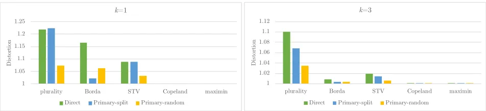
Figure 1: The distortion values for various settings (Direct, Primary-split and Primary-random) and voting rules fork∈ {1,3}. Each bar represents the average distortion over1000instances. Within each figure, all of the bars represent average distortion over the same set of voter and candidate locations, but not necessarily party affiliations. ANOVA on all elections returned
p <10−9whenk= 1andp <10−5whenk= 3
Using Simulations to Go Beyond Worst Case
So far we compared the distortion of a voting rule under the direct and primary systems, taken in theworst caseover a family of instances. In practice, such worst case instances may not arise naturally. In this section, we compare the dis-tortion of a voting rule under the direct and primary systems, in theaverage caseover simulated instances. To control for the effect of vastly different numbers of voters or candidates affiliated with the two parties, we place the restriction that half of the voters and half of the candidates must be affiliated with each party. Furthermore, we wish to examine instances in which voters and candidates affiliated with one party are separated from those affiliated with the other party.We fix the metric space to be[0,1]kfork∈ {1,3,5,7,9}
with the Euclidean distance. We generate1000instances sat-isfying the following restrictions. First, we place a setV of
n = 1000voters at uniformly random locations in[0,1]k.
Next, we find a hyperplane dividing voters into two equal halves. Due to symmetry, we simply find a thresholdt on thekthcoordinate such that the locations of half of the
vot-ers (call this setV−1) have a smaller kth coordinate, while
the locations of the rest (call this setV1) have a greaterkth
coordinate. We do not affiliate the voters yet. Next, we place
m
2 = 10candidates (call this setA−1) uniformly at random on one side of the hyperplane, andm2 = 10candidates (call this setA1) uniformly at random on the other side.
Once the locations of the voters and candidates are fixed, we create two instances. In one instance (“split”), we as-signV−1∪A−1to party−1, and assignV1∪A1to party
1. This instance belongs toI0.5
m,sep-Rk. In the other instance
(“random”), we assign half of the voters and half of the can-didates chosen uniformly at random to party−1, and the rest to party1. This instance belongs toI0.5
m,Rk, but not
necessar-ily toI0.5
m,sep-Rk. This allows us to directly compare the
ef-fect that separability has on the distortion. Finally, we run five voting rules — plurality, Borda, STV, Copeland and maximin — on both instances under the direct and primary systems, and measure the distortion. Note that their distor-tion under the direct system would be identical for both in-stances because the two inin-stances only differ in party affili-ations. Thus, for each rule, we obtain three numbers: Direct,
Primary-split, and Primary-random. We average the distor-tion numbers across the1000instances.
See Figure 1 for selected simulation results. The results fork > 3resemble those fork = 3in their comparison of the direct versus the primary system; the only difference is that the overall distortions are lower for higherk. To com-pare the three distortion numbers in each case, we ran a re-peated measures ANOVA comparing the distortion values, and in all but 2 of 25 cases, had apvalue under0.05(the two cases hadk= 9).
Perhaps the most important observation is that our simula-tion results stand in direct contrast to our worst-case bounds. In almost all of our settings, the distortion under the pri-mary system (split and random) is better than that the distor-tion under its direct counterpart, and often shows a signifi-cant improvement. This is especially noticeable in the non-Condorcet consistent rules (plurality, Borda and STV), as in all but 3 of 15 cases the distortion significantly improves the primary system in both cases. This effect is most pro-nounced with plurality. With Condorcet consistent rules, the distortion values are very low, regardless of whether the di-rect system is used or the primary system. In general, as we increase the dimensionk, the groups become more homoge-nous and thepvalues grow, while distortions approach1.
Overall, the simulation results show a distortion that is far below our theoretical worse-case results. We suspect that the reason for this difference might have to do with our choice of uniform voter and candidate distributions, and distortion numbers might differ under different distributions.
Discussion
Our paper initiates the novel quantitative study of multi-stage elections (and their comparison to single-multi-stage elec-tions), but leaves plenty to explore. Some directions are fairly straightforward extensions of our results. The most straightforward question is to tighten our bounds. There is also the question of explaining the trends we observe in the average case, which sometimes differ from our worst-case results. A next step would be to study realistic distributional models of voter preferences and candidate positions in the political spectrum, and analyze their effect on distortion.
our framework to more than two parties requires the use of a ranked voting rule in the general election, which may signif-icantly affect the analysis. Interestingly, such an extension would also incorporate independent candidates because one can imagine an independent candidate to be a party of their own. Examining the use of multiple and different voting rules as Narodytska and Walsh (2013) do for two-step voting (though without candidate elimination between stages) is an enticing direction. For example, in a multi-party direct sys-tem, we may use plurality, whereas in the primary syssys-tem, the parties may use STV. It is also reasonable to consider that each party has its own voting rule. It would be inter-esting as well to examine party manipulation techniques in primary systems. Similarly, it is reasonable to believe that candidates may also strategically shift, to some extent, their location following the primaries, to make themselves more appealing to the general electorate.
We believe that the study of multi-stage elections and party mechanisms can not only contribute novel theoretical challenges to tackle, but can also bring research on computa-tional social choice closer to reality and increase its impact.
Acknowledgements
This work was partially supported by NSERC under the Dis-covery Grants program.
References
Anshelevich, E., and Postl, J. 2017. Randomized social choice functions under metric preferences. Journal of Artificial Intelli-gence Research58(1):797–827.
Anshelevich, E.; Bhardwaj, O.; and Postl, J. 2015. Approximating optimal social choice under metric preferences. In29th, 777–783. Bartholdi III, J. J.; Tovey, C. A.; and Trick, M. A. 1992. How hard is it to control an election?Mathematical and Computer Modelling 16(8–9):27–40.
Black, D. 1948. On the rationale of group decision-making. Jour-nal of Political Economy56:23–34.
Boutilier, C.; Caragiannis, I.; Haber, S.; Lu, T.; Procaccia, A. D.; and Sheffet, O. 2015. Optimal social choice functions: A utilitarian view.Artificial Intelligence227:190–213.
Brandt, F.; Conitzer, V.; Endriss, U.; Lang, J.; and Procaccia, A. D., eds. 2016.Handbook of Computational Social Choice. Cambridge University Press.
Brill, M., and Conitzer, V. 2015. Strategic voting and strategic candidacy. In29th, 819–826.
Cohen, M.; Karol, D.; Noel, H.; and Zaller, J. 2008. The Party Decides: Presidential Nominations Before and After Reform. Uni-versity of Chicago Press.
Cohensius, G.; Mannor, S.; Meir, R.; Meirom, E.; and Orda, A. 2017. Proxy voting for better outcomes. In16th, 858–866. Conitzer, V., and Yokoo, M. 2010. Using mechanism design to prevent false-name manipulations.AI Magazine31(4):65–77. Cross, W. P., and Blais, A. 2011. Who selects the party leader? Party Politics18(2):127–150.
Cross, W. P., and Katz, R. S., eds. 2013. The Challenges of Intra-Party Democracy. Oxford University Press.
Downs, A. 1957.An Economic Theory of Democracy. Harper and Row.
Dutta, B.; Jackson, M. O.; and Le Breton, M. 2001. Strategic candidacy and voting procedures.Econometrica69(4):1013–1037. Dutta, B.; Jackson, M. O.; and Le Breton, M. 2002. Voting by suc-cessive elimination and strategic candidacy. Journal of Economic Theory103(1):190–218.
Feldman, M.; Fiat, A.; and Golomb, I. 2016. On voting and fa-cility location. In Proceedings of the 17th ACM Conference on Economics and Computation (EC), 269–286.
Hamilton, A.; Madison, J.; and Jay, J. 1787.The Federalist Papers. The Independent Journal.
Hazan, R. Y. 1997. The 1996 intra-party elections in israel: Adopt-ing party primaries.Electoral Studies16(1):95–103.
Jobson, R., and Wickham-Jones, M. 2010. Gripped by the past: Nostalgia and the 2010 labour party leadership contest. British Politics5(4):525–548.
Kahng, A.; Mackenzie, S.; and Procaccia, A. D. 2018. Liquid democracy: An algorithmic perspective. In32nd, 1095–1102. Kenig, O. 2009. Classifying party leaders’ selection methods in parliamentary democracies. Journal of Elections, Public Opinion and Parties19(4):433–447.
Narodytska, N., and Walsh, T. 2013. Manipulating two stage voting rules. In12th, 423–430.
Norpoth, H. 2004. From primary to general election: A forecast of the presidential vote. PS: Political Science & Politics37(4):737– 740.
Polukarov, M.; Obraztsova, S.; Rabinovich, Z.; Kruglyi, A.; and Jennings, N. R. 2015. Convergence to equilibria in strategic can-didacy. In24th, 624–630.
Procaccia, A. D., and Rosenschein, J. S. 2006. The distortion of cardinal preferences in voting. InProceedings of the 10th In-ternational Workshop on Cooperative Information Agents (CIA), 317–331.
Rothe, J., ed. 2015.Economics and Computation. Springer. Schofield, N. 2008. The Spatial Model of Politics. Number 95 in Routledge Frontiers of Political Economy. Routledge.
Sides, J.; Tausanovitch, C.; Vavreck, L.; and Warshaw, C. 2018. On the representativeness of primary electorates. British Journal of Political Science1–9.
Simms, B. 2007.Three Victories and a Defeat: The Rise and Fall of the First British Empire, 1714-1783. Allen Lane.
Skowron, P., and Elkind, E. 2017. Social choice under metric preferences: Scoring rules and stv. InProceedings of the 31st AAAI Conference on Artificial Intelligence (AAAI), 706–712.
Wauters, B. 2010. Explaining participation in intra-party elections: Evidence from belgian political parties. Party Politics16(2):237– 259.