Volume -3, Issue-1, January – February 2017, Page No. 01 - 13
e1
ISSN: 2455 - 1597
Robost Video Object Segmentation and Feature Extraction Using Thresholding Technique
K.Aparna1, S.Swarna Latha2
1
S.V University, Department of E.C.E, Tirupati, Chittoor District, A.P
E-Mail Id: [email protected]
2
Associate, S.V. University, Department of E.C.E, Tirupati, Chittoor District, A.P
E-Mail Id: [email protected]
Abstract
In this paper, we present a novel bottom-up salient object detection approach by exploiting the relationship between the
saliency detection and the Markov absorption probability. First, we calculate a preliminary saliency map by the Markov
absorption probability on a weighted graph via partial image borders as background prior. Unlike most of the existing
background prior-based methods which treated all image boundaries as background, we only use the left and top sides as
background for simplicity. The saliency of each element is defined as the sum of the corresponding absorption probability
by several left and top virtual boundary nodes, which are most similar to it. Second, a better result is obtained by ranking
the relevance of the image elements with foreground cues extracted from the preliminary saliency map, which can
effectively emphasize the objects against the background, whose computation is processed similarly as that in the first
stage and yet substantially different from the former one. At last, three optimization techniques—content-based diffusion
mechanism, super pixel wise depression function, and guided filter—are utilized to further modify the saliency map
generalized at the second stage, which is proved to be effective and complementary to each other. Both qualitative and
quantitative evaluations on four publicly available benchmark data sets demonstrate the robustness and efficiency of the
proposed method against 17 state-of-the-art methods. Our method exploits features of colour and luminance, is simple to
implement, and is computationally efficient. In our proposed work salient feature based segmentation will be based on
contrast, gradient, illumination, edges and gradients, spatial frequencies, structure and distribution of image patches,
histograms, multi-scale descriptors. The saliency features will be extracted by applying Histogram of Gradient (HoG) and
Difference-of-Gaussian (DoG) detector. A common approach is to use fuzzy iterative clustering algorithms that provide a
partition of the pixels into a given number of clusters. To segment the ROI (Region of Interest), the algorithm is
developed by modifying the objective function of the standard FCM algorithm with a penalty term that takes into account
the influence of the neighboring pixels on the centre pixels.
Keywords: Content-Based Diffusion, Super Pixel Wise Depression Function, And Guided Filter
1. Introduction
Saliency detection plays an important role in a variety of applications including salient object detection, salient object
segmentation, content-aware image/video retargeting, content-based image/video compression, and content-based image
retrieval, etc. Generally, saliency is defined as what captures human perceptual attention. Human vision system (HVS) has
the ability to effortlessly identify salient objects even in a complex scene by exploiting the inherent visual attention
mechanism. With the goal both to achieve a comparable saliency detection performance of HVS and to facilitate different
e2 e2 e2 e2 e2 e2 e2 e2 e2
e2
e2
e2
e2 e2 e2 e2 e2 e2 e2 e2
e2
proposed in the past decades, and a recent benchmark for saliency models on saliency detection performance is reported.
The early research on saliency model is motivated by simulating the visual attention mechanism of HVS, through which
only the significant portion of the scene projected onto the retina is thoroughly processed by human brain for semantic
understanding. Based on the biologically plausible visual attention architecture and the feature integration theory, Itti et al.
proposed a well-known saliency model, which first computes feature maps of luminance, colour and orientation using a
center-surround operator across different scales, and then performs normalization and summation to generate the saliency
map. Salient regions showing high local contrast with their surrounding regions in terms of any of the three features are
highlighted in the saliency map. Since then, the center-surround scheme has been widely exploited in a variety of saliency
models, due to its clear interpretation of visual attention mechanism and its concise computation form. The
centre-surround scheme is implemented using a number of features including local contrasts of colour, texture and shape
features, oriented subband decomposition based energy, ordinal signatures of edge and colour orientation histograms,
Kullback-Leibler (KL) divergence between histograms of filter responses , local regression kernel based self-resemblance,
and earth mover’s distance (EMD) between the weighted histograms. The selection of surrounding region is the key factor
to suitably evaluate the saliency of the center pixel/region. Rather than using a fixed shape such as rectangle or circular
region, the surrounding region is selected as the whole region of the blurred image in the frequency-tuned saliency model,
and the maximum symmetric region.
2. Existing System
Edge based Region Growing is an approach to image segmentation in which neighboring pixels are examined and added
to a region class if no edges are detected. This process is iterated for each boundary pixel in the region. If adjacent regions
are found, a region-merging algorithm is used in which weak edges are dissolved and strong edges are left in tact.
a. Disadvantages of Existing System
1. The region growing segmentation is not preferred for its limited range of applications and automatic features are not
having accurate values.
2. Pre-processing experiments are needed to find which type of filtering will be more beneficial. This increases the effect
of the speckle noise and Gaussian noise the in the image.
Proposed Block Diagram
Figure-1: Block diagram for video object segmentation and feature extraction
3. Proposed Algorithm
e3 e3 e3 e3 e3 e3 e3 e3 e3
e3
e3
e3
e3 e3 e3 e3 e3 e3 e3 e3
e3
1. Enhanced Adaptive Hybrid Median Filter
Enhanced Adaptive Hybrid Median filtering is similar to an averaging filter, in that each output pixel is set to an average
of the pixel values in the neighborhood of the corresponding input pixel. However, with median filtering, the value of an
output pixel is determined by the median of the neighborhood pixels, rather than the mean. The median is much less
sensitive than the mean to extreme values (called outliers). Median filtering is therefore better able to remove these
outliers without reducing the sharpness of the image.
2. Saliency Feature Extraction using HoG (Histogram of Gradient)
We compute Histograms of Oriented Gradients (HOG) to describe the distribution of the selected edge points. HOG is
based on normalized local histograms of image gradient orientations in a dense grid. The HOG descriptor is constructed
around each of the edge points. The neighborhood of such an edge point is called a cell. Each cell provides a local 1-D
histogram of quantized gradient directions using all cell pixels. To construct the feature vector, the histograms of all cells
within a spatially larger region are combined and contrast-normalized.
3. Modified Fuzzy C Means algorithm with Expectation Maximization clustering technique
First, we calculate the image saliency by using the colour and space information of both local and global in single scale.
Then by applying the multi-scale fusion, we can effectively inhibit outstanding but not salient region in each single scale,
and different scale can also reflect salient region of the images from different aspects. Many image display devices allow
only a limited number of colours to be simultaneously displayed. Usually, this set of available colours, called a colour
palette, may be selected by a user from a wide variety of available colours. Such device restrictions make it particularly
difficult to display natural colour images since these images usually contain a wide range of colours which must then be
quantized by a palette with limited size. This colour quantization problem is considered in two parts: the selection of an
optimal colour palette and the optimal mapping of each pixel of the image to a colour from the palette. The entire work is
divided into two stages. First enhancement of colour separation of satellite image using de-correlation stretching is carried
out and then the regions are grouped into a set of five classes using Fuzzy c-means clustering algorithm. Using this two
step process, it is possible to reduce the computational cost avoiding feature calculation for every pixel in the image.
Although the colour is not frequently used for image segmentation, it gives a high discriminative power of regions present
in the image.
b. Advantages of Proposed System
1. It is the fastest algorithm when compared to the k means algorithm and modified Fuzzy C Means algorithm.
2. The proposed anisotropic diffusion filter will completely eliminates the speckle noise from the image.
3. The proposed algorithm is applicable for RGB colour space images.
4. We were able to successfully apply a segmentation method based on Expectation Maximization clustering.
5. The use of saliency promises benefits to multimedia applications.
e4 e4 e4 e4 e4 e4 e4 e4 e4
e4
e4
e4
e4 e4 e4 e4 e4 e4 e4 e4
e4
4.1. Object Tracking Techniques
a. Gray Scales Feature
Gray Scale feature is the histogram of the given image in the gray format.
b. HoG (Histogram of Gradient)
We compute Histograms of Oriented Gradients (HOG) to describe the distribution of the selected edge points. HOG is
based on normalized local histograms of image gradient orientations in a dense grid. The HOG descriptor is constructed
around each of the edge points. The neighborhood of such an edge point is called a cell. Each cell provides a local 1-D
histogram of quantized gradient directions using all cell pixels. To construct the feature vector, the histograms of all cells
within a spatially larger region are combined and contrast-normalized.
c.LBP (Local Binary Pattern)
The local binary pattern operator is an image operator which transforms an image into an array or image of integer labels
describing small-scale appearance of the image. These labels or their statistics, most commonly the histogram, are then
used for further image analysis. The most widely used versions of the operator are designed for monochrome still images
but it has been extended also for color (multi channel) images as well as videos and volumetric data.
d. GLCM (Gray Level Co-occurance Matrix)
The Following GLCM features were extracted in our research work: Autocorrelation, Contrast, Correlation, Cluster
Prominence, Cluster Shade, Dissimilarity Energy, Entropy, Homogeneity, Maximum probability , Sum of squares, Sum
average, Sum variance, Sum entropy, Difference variance, Difference entropy, Information measure of correlation,
information measure of correlation, Inverse difference normalized.
e. Object Tracking using SVM classifier with Kalman Filter
The system is fully automatic and requires no manual input of any kind for initialization of tracking. Through establishing
Kalman filter motion model with the features centroid and area of moving objects in a single fixed camera monitoring
scene, using information obtained by detection to judge whether merge or split occurred, the calculation of the cost
function can be used to solve the problems of correspondence after split happened. The algorithm proposed is validated on
human and vehicle image sequence.
The MVS tracker is implemented under the Kalman filter framework and employs different views of features to train
corresponding SVMs respectively. We present how to implement the appearance model with multi-view SVMs to
represent the object, and then introduce the entropy strategy, which is used to combine the multi-view SVMs and
embedded into the Kalman filter framework to determine the tracking results. Besides, we describe the subspace evolution
e5 e5 e5 e5 e5 e5 e5 e5 e5
e5
e5
e5
e5 e5 e5 e5 e5 e5 e5 e5
e5
4.2. Crowd Tracking Techniques
a. Motion Pixel Estimation
Finding gradients: The edges should be marked where the gradients of the image has large magnitudes.
Non-maximum suppression: Only local maxima should be marked as edges.
Double thresholding: Potential edges are determined by thresholding.
Edge tracking by hysteresis: Final edges are determined by suppressing all edges that are not connected to a very certain
(strong) edge.
b. Crowd tracking using FAST algorithm
One of the key aspects of crowd tracking is feature extraction. Under the assumption that regions of low density crowd
tend to present less dense local features compared to high-density crowd, we propose to use local features as a description
of the crowd by relating dense or sparse local features to the crowd size. For local features, we assess Features from
Accelerated Segment Test (FAST). FAST is proposed for corner detection in a fast and a reliable way. It depends on
wedge model style corner detection. Also, it uses machine learning techniques to find automatically optimal segment test
heuristics.
5. Results
Figure-2: Effective object discovery from multiple videos even with some frames not containing the common object.
The first row shows two related video sequences and the common object plane does not appear in every frame. The
object-like area of each frame estimated through [10] is presented in the second row. The bottom row shows the more
correct object discovery results through [13] with further utilizing the inter-frame consistence property. Those frames with the ratio κ ≤ 0.2 are considered not to contain the common object, which are marked in the red rectangles.
Effective object discovery from multiple videos even with some frames not containing the common object. The first row
shows two related video sequences where the common object plane does not appear in every frame. The object-like area
e6 e6 e6 e6 e6 e6 e6 e6 e6
e6
e6
e6
e6 e6 e6 e6 e6 e6 e6 e6
e6
discovery results through [13] with further utilizing the inter-frame consistence property. Those frames with the ratio κ ≤
0.2 are considered not to contain the common object, which are marked in the red rectangles.
There are many videos that include frames that do not contain the common object (e.g. the first row of Figure-5). Current
video co-segmentation approaches disregard this challenge and assume common object appears in every frame. Our
method effectively handles this difficulty. One intuition is that the frames that do not contain the common object are not
consistent with the frames that contain the object. Therefore, we further leverage the inter-frame consistency property.
Based on [10], we get object-like areas and background areas for each frame. Suppose frame fnk-1contains the common
foreground while does not. Their estimated object-like area should be different. We employ Gaussian mixture models
(GMM) to characterize the common object appearance. For frame the GMMs for object-like area and background
are defined as respectively.
Figure- 3: Overview of our object refinement stage on frame and frame . (a) After object discovery step, a pair of
videos is randomly selected to perform object refinement. (b) Object-like area is obtained after the object discovery step.
(c) Visualization of spatio-temporal SIFT flow field. The discontinuities of spatio-temporal SIFT flow field reveal the
variation of object structure. (d) Result of over-segmentation on spatio-temporal SIFT flow field. (e) A more accurate
object partitioning is obtained by removing the pixels that are similar to background. (f) GMM for kth frame is updated
based on the updated estimation in (e).
We introduce an object consistence term to measure the consistency of estimated objects in video according to the
e7 e7 e7 e7 e7 e7 e7 e7 e7
e7
e7
e7
e7 e7 e7 e7 e7 e7 e7 e7
e7
Where denotes the probability of pixel x for foreground, which is obtained from of prior
frame .
Then we add this object consistence term into our object discovery energy function:
We set parameter for all the test videos in our experiments. Since five or ten frames between frame
and , the estimated GMM for frame is helpful for identifying whether the frame contains the common
object. From Fig. 5 we see that the object discovery energy function in (13) is a better choice for detecting the frames not
containing common object due to the inter-frame consistency.
We use to denote the object-like area in frame and the number of pixels belonging to the object-like area Tkn is
expressed as . We consider whether frame f k n contains the common object in case the ratio
is relatively large and conclude that the foreground object of frame is not changed. Conversely, if this ratio
is small, we assume the objects between frames and are not consistent. In this case, frame is considered to not
contain the common object and we set . The GMM of the frame is set as:
In this way, the GMM for common object is kept consistent across the whole video sequence by ignoring the ‘noise’
frames. The frames that are detected to not contain the objects in object discovery step, will be not taken into
consideration in next object refinement process.
1.Object Tracking
Upon obtaining a fairly accurate representation of where moving objects lie in a given video frame, it is possible to
segment the foreground layer further and isolate each individual object as its own entity. A term developed from a
previous application that tracks moving bodies [4] in a video sequence is borrowed that encompasses the spirit of how
these object should be regarded. Each object is treated as a “blob” where all points within are connected.
Each one of these entities can be tracked by finding its center of gravity. This can be interpreted as the spatial center of
each blob. A rough estimate of the trajectory of the blob can be computed by finding a translational motion estimate
based on the change of position from one frame to another using an 8x8 block centered at the centroid of the blob. This is
e8 e8 e8 e8 e8 e8 e8 e8 e8
e8
e8
e8
e8 e8 e8 e8 e8 e8 e8 e8
e8
Figure-4: Object tracking
Input Videos K means (Existing System) PSNR in dB
FCM (Existing System)
PSNR in dB
MFCM (Proposed System) PSNR in dB
Bird 28 36 43
Boat 27 34 40
Car 29 38 44
Cat 27 34 40
Moto 23 29 38
Plane 26 35 42
Mean Square Error
Input Videos K means (Existing System) PSNR in dB
FCM (Existing System)
PSNR in dB
MFCM (Proposed System) PSNR in dB
Bird 100 8 0.0001
Boat 111 10 0.001
Car 90 7 0.00001
Cat 111 10 0.001
Moto 150 12 0.01
Plane 105 11 0.0004
2. Algorithm Details
In this paper we chose a three-step process to segment upright moving people from the campus scenes. The first step
e9 e9 e9 e9 e9 e9 e9 e9 e9
e9
e9
e9
e9 e9 e9 e9 e9 e9 e9 e9
e9
[1]. To simplify the computational complexity of the mixture models, grayscale images were used instead of the three
independent color channels as first proposed in the paper. After converting the original color images to grayscale, the
algorithm determines the background and foreground pixels and outputs a binary representation of the foreground. The
second step involved computing connected components from the binary video to determine significant regions of interest
based on area. The third step involved a high level analysis of the interesting regions found in step two. The output of
this step resembles binary motion blobs. A recursive technique was performed on the binary motion blobs of step two to
distinguish upright, moving people from large object scene clutter.
For each of these steps there is a determination of the types of parameters to be used, each of which will be expounded
upon in detail in the coming sections. The online mixture model requires three parameters: the number of Gaussian
mixture models, the adaptation constant and the minimum percentage of background to be accounted for by the models.
There are two remaining parameters used during the high level analysis to determine the upright, moving people in the
scene: minimum area and height of people in the scene. In general, we found these two groups of parameters to remain
very similar among different scenes of similar types of video (people moving in campus scenes). It is believed that in
other scenarios they could be tweaked to provide adequate performance.
3. Initial Foreground Segmentation via Motion Cues
The foreground was initially segmented using the Gaussian Mixture Model presented in [1]. The authors chose this
method because of its demonstrated efficacy and computational efficacy. These two factors have led to the methods wide
acceptance among researchers in the computer vision community.
This segmentation method works by modeling each pixel by a mixture of Gaussian distributions. Each Gaussian is
assigned a weight based on its likelihood to be a good model for the background. This is accomplished by weighting
each of the Gaussians by how frequently they are observed in the past. This weight is an average with an exponentially
decaying window. Specifically, each mixture’s weight is updated in the following manner:
) ( )
1
( , 1 ,
,t kt kt
k
α
ω
α
Mω
= − − + , (1)Where ωk,t is the weight for the kthmixture at time t and α is the “learning coefficient” that controls how long previously seen mixture components remain in “memory”. For the specific results shown in the following sections, α was set to 0.001 while k, the number of Gaussian mixtures was set to 4.
When a pixel is observed that does not belong to any of the existing mixture models it is most likely a “foreground”
pixel. However, if it remains constant for long enough it can be incorporated into the background. Therefore if a new
pixel is not within a certain amount of standard deviations of the existing mixtures, a new mixture is created replacing the
least likely prior mixtures with arbitrarily high mean and variance (while the new mean and variance are arguably more
tuning parameters for this method we view them as not as significant as the other parameter selections of this approach).
e10 e10e10 e10e10 e10e10 e10e10
e10
e10
e10
e10e10 e10e10 e10e10 e10e10
e10
background pixels are determined by ordering the Gaussians by weight and accounting for the minimum amount of data
representing the background (T),
>
=
∑
= b
k k
b
T
B
1
min
arg
ω
. (2)The minimum portion of the data that should be accounted for by background, T, is set to be 0.5 in scenes that are
depicted in the following sections.
Typically the Gaussian mixture model requires an initial representation of the background. For the scenes analyzed, the
algorithm provides adequate results without the need training data. In this way, the authors do not calculate an initial
probabilistic representation of the image background. In fact, ‘training’ the Gaussians with ten averaged frames of the
entire scene does not provide significantly better results. The difference in segmentation between the methods is nearly
imperceptible.
4. Connected Component Analysis
Eight-way connected component analysis was performed on each binary image resulting from the output of the Gaussian
mixture model. Binary blobs smaller than an area threshold were removed from the image. For the following
segmented images the minimum area that would constitute a person was set to be 550 pixels.
High Level Analysis
A recursive technique was performed on the binary motion blobs of step two to distinguish upright, moving people from
large object scene clutter. Mainly, an ‘upright, moving person’ was discriminated by height in addition to area. The
height threshold of a person was set to be 30 pixels.
In many cases, the people in the scene were joined by their shadow to create one large connected component blob. To
remove the shadow portion of the connected blob and to discriminate between the two people, height was used. This was
done by summing down the binary columns of each connect blob matrix to form a vector. The assumption of upright
people is now exercised as we remove columns in the blob which have values less than our height threshold. The
shadows had a low height and the upright person had a large height. A threshold was used to distinguish the two. When
two people were attached by one connected blob through one of their shadows, it is necessary to determine where break
the two apart. Because of this, a recursive approach was used by which each blob was broken into fundamental parts and
then each of those parts was analyzed until a base case was reached. The base case blob met the area and height
requirements.
The recursive approach worked by first performing connected component analysis on a morphological dilation of the
e11 e11e11 e11e11 e11e11 e11e11
e11
e11
e11
e11e11 e11e11 e11e11 e11e11
e11
This process was then repeated for the resulting blobs until a steady state was reached for a given frame. The blobs
remaining become the final segmentation.
5. Evaluation
In this paper we choose a standard set of campus video sequences encoded in MPEG format. The scenes feature students
walking, sitting, and bicycle riding. Given an initial motion cue, we wish to segment an individual for the remainder of
the scene regardless of their motion or lack of motion. We wish to distinguish between human motion and motion of
other objects such as vegetation movement (wind) and other background distracters.
As an additional metric, we seek to determine the number of individuals present in a scene. This leads to the desires of a
real-time tracking system in which the numbers of individuals present in the scene is a fundamental requirement. We
determine the number of individuals in the scene by determining the number of total objects in the scene after the
recursive algorithm has broken apart connected human objects.
As a measure of comparison we compare our higher-level processing with that of the Expectation Maximization (EM)
algorithm as presented in [Forsyth, Ponce]. The EM algorithm is performed on objects enclosed by blobs that meet our
height/area requirements. It is performed in the smallest rectangular bounding box about the blob. Two regions are used
in the segmentation with the assumption of a background region with a normal distribution and a different foreground
region with a separate normal distribution. The initial mean and variance of each is computed from the first guess as to
where the person is in the scene. This guess corresponds to the binary mask of foreground pixels from the Gaussian
mixture model. The EM algorithm then iterates until convergence. In the images of Error! Reference source not
found., it can be seen that in some instances it provides very good results. But in others, it is seen that the EM
completely fails. This is because the gray values are far from the assumption in the EM algorithm of two very different
homogenous regions constituting the foreground and background. Additional filtering could be done to try to mitigate
these problems and force the EM algorithm to converge to better results (vertical smoothing of the image would result in
more homogenous regions). Nevertheless, the straightforward EM segmentation as proposed in [2] yields results that
when they converge are comparable to those of the CAMPUS method, however it is ineffective in converging in nearly
half the frames for all of the people in the scene that the CAMPUS algorithm detects.
An important metric in the evaluation of the CAMPUS algorithm the computational efficiency. For 320x240 images the
throughput of the CAMPUS algorithm is 125 frames/minute as coded in MATLAB on a 1Ghz Pentium Celeron with
512MB RAM running Windows XP. In comparison the EM based segmentation provides 115 frame/minute throughput
on the same hardware.
Two campus scenes were analyzed using the algorithm. These scenes involve students walking in and out of the
e12 e12e12 e12e12 e12e12 e12e12
e12
e12
e12
e12e12 e12e12 e12e12 e12e12
e12
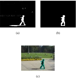
The first scene, old main, depicts students sitting in the grass and walking on a sidewalk. The algorithm successfully
segments the upright, walking people and does not include those sitting in the grass. Table 1 displays a selected frame
from the results.
(a) (b)
(c)
Table 1. Depiction of segmentation steps of oldmain video. (a) Initial segmentation via Gaussian mixture model algorithm. (b) High level segmentation via our recursion technique. (c) An overlay of the segmentation onto the colored frame.
6. Conclusion
We presented a robust video co-segmentation method that discovers the common object over an entire video dataset and
segments out the objects from the complex backgrounds. Saliency, motion cues and SIFT flow are integrated into our
spatio-temporal SIFT flow to explore the relationships between foreground objects. Furthermore, we formulate the video
co-segmentation problem as an object optimization process, which progressively refine the estimation for object in three
steps: object discovery, object refinement and object segmentation. Both the quantitative and qualitative experimental
results have shown that the proposed algorithm creates more reliable and accurate video co-segmentation performance
than the state-of-the-art algorithms. Unlike previous work, we emphasize that object discovery process should be robust to
foreground variations in appearance or motion patterns, which extends the applicability of our co-segmentation method.
7. References
[1] H. Barlow. Possible Principles Underlying the Transformation of Sensory Messages. Sensory Communication, pages 217–234, 1961. 1
[2] H. Egeth, R. Virzi, and H. Garbart. Searching for Conjunctively Defined Targets. Journal of Experimental psychology:
e13 e13e13 e13e13 e13e13 e13e13
e13
e13
e13
e13e13 e13e13 e13e13 e13e13
e13
[3] R. Fergus, P. Perona, and A. Zisserman. Object class recognition by unsupervised scale-invariant learning. Proc. CVPR, 2, 2003.
[4].J. Gluckman. Order Whitening of Natural Images. Proc. CVPR, 2, 2005. [5] J. Intriligator and P. Cavanagh. The Spatial Resolution of Visual Attention. Cognitive Psychology, 43(3):171–216, 2001.
[6] L. Itti and C. Koch. A Saliency-Based Search Mechanism for Overt and Covert Shifts of Visual Attention. Vision