ISSN 1392–124X (print), ISSN 2335–884X (online) INFORMATION TECHNOLOGY AND CONTROL, 2016, T. 45, Nr. 4
Continuous-Time Delay-Petri Nets as A New Tool to Design
State Space Controller
Alireza Ahangarani Farahani, Abbas Dideban
1Semnan University, Department of Electrical and computer Engineering, Semnan, Iran
e-mail: [email protected]
http://dx.doi.org/10.5755/j01.itc.45.4.13665
Abstract. In this paper a new method of modelling and controller design for continuous systems is introduced. Petri Net is a useful tool for modelling, analysis and controller synthesis in discrete event systems. Continuous-Time Delay-Petri Nets (CTDPN) are presented to challenge with other types of continuous dynamic system modelling tools. This article focuses on an approach to design a controller using Petri Net for continuous dynamic systems. It is shown here that this method simplifies system analysis and controller design by first, converting the continuous state space to a discrete state space and then applying CTDPN, to model and analyse it. Finally, a state feedback control algorithm is adapted to be used for models which are derived by CTDPN approach. Simulation results show the efficiency of the proposed approach comparing to state space feedback controller in terms of the simplicity of the system analysis and the time it takes to simulate the close-loop system.
Keywords: Continuous Petri Nets; Controller Design; State Feedback; Time Delay Petri Nets.
1. Introduction
Recently, due to great advances in technology and computer aided techniques, modelling based on Petri Nets has attracted researchers’ attention. Automata and Petri Nets are the main modelling tools in the area of control synthesis for discrete event systems in compu-ter integrated manufacturing systems, correspondence, aviation, spaceflight, etc. In the last decade, many researchers study modelling based on Petri Nets because of the advantages of the graphical and distributed representations of the system states and the computational efficiencies [1,2].
Petri Nets have been used extensively as a tool for modelling, analysis and synthesis of discrete event systems and usually interpreted as a control flow graph of the modelled system [3]. This method is an alternative tool for modelling event based systems [4]. Petri Nets are both a graphical and mathematical tool that can model deterministic or stochastic system behaviours and phenomena such as parallelism, asynchronous behaviour, conflicts, resource sharing and mutual exclusion [5].
Petri Nets were introduced in Carl A. Petri’s 1962 Ph.D. dissertation [6]. Since then, researches have proved it to be a helpful graphical and mathematical modelling tool applicable to many systems. As a graphical tool, Petri Nets can be used as an effective
visual communication aid similar to flow charts, block diagrams, and networks [6]. As a mathematical tool, the modelling procedure based on Petri Nets can describe the system behaviour by linear algebraic equations [7].
Continuous Petri Nets model was presented by David and Alla in [8]. These authors have obtained a continuous model by fluidization of a discrete Petri Nets [9]. This approach is a useful method for modelling of many phenomena and systems. In [10], controllability of Timed Continuous Petri Nets, under infinite server semantics, with uncontrollable transitions is presented. Further, Continuous Petri Nets constitute a part of process of modelling by a systematic procedure that was discussed in [11]. The continuous part can model systems with continuous flows. Autonomous Continuous Petri Nets and other models like Differential Algebraic Equations Petri Nets have been studied intensively in this research area [12, 13]. Digitized signals leaning on analogue signal and continuous approximated model are used in this paper which presents important connection between mathematical transfer function and state event base model [14]. This leads to a mathematical model with very simple algorithm in contrast with the complexity of mathematical models.
usually expressed as a transfer function and never use any knowledge of the interior structure of the plant.
Modern control theory solves many of the limita-tions by using a much richer description of the system dynamics. The so-called state space description represents the dynamics as a set of coupled first-order differential equations between a set of internal variables known as state variables, together with a set of algebraic equations that combine the state variables into physical output variables [15].
For many systems, the differential equations of the system change due to the change of conditions. Hence, there are different transfer functions and the system can be divided into a number of subsystems. Therefore, they are absolutely difficult to be modelled and controlled. One of the most powerful tools to model and control these types of systems is Petri Nets. Some previous attempts are done in order to model continuous dynamic systems using Petri Nets [16].
Here in this article a Continuous-Time Delay-Petri Nets (CTDPN) method is presented to solve the difficulty of modelling and control. Using CTDPN, first continuous state space is modelled by Petri Nets approach. After modelling step, a state feedback control algorithm based on CTDPN is introduced. One of the significant advantageous of this procedure is that all features of the system are preserved in incidence matrix.
The remainder of this paper is organized as follows: In Section 2, main concepts of discrete and continuous Petri Nets are presented. The basic definitions for Continuous-Time Delay-Petri Nets (CTDPN) are explained in Section 3. The differences between CTDPNs with PNs are also explained in this section. The control algorithm based on state space controller is presented in Section 4. Section 5 is dedicated to simulation results and finally the conclusion is stated in Section 6.
2. Basic Concepts and Notations
2.1. Ordinary Petri Nets
Petri Net is a directed net consisting of places, transitions, directed arcs and tokens [17].
A Petri Net is a 5-tuple N = {P, T, W-(Pre), W+(Post), M
0} where:
P= {p1, p2,…, pn} is a finite set of places, and n>0
is the number of places;
T= {t1, t2,…, tm} is a finite set of transitions, and m>0 is the number of transitions and P∩T=Ø, i.e. the sets P and T are disjoint;
Pre or W-: (P×T) →N is the input function, Post or W+:(T×P) →N is the output function;
M0 is the initial marking. The incidence matrix W is calculated by W=W+- W-.
Pictorially, places are represented by circles, transitions are represented by rectangles or bars, and arcs are depicted as arrows.
Here, the following notations will be used [18]:
Pr , 0
o
j j
t piP e p ti = set of input places of tj.
P , 0
j pi P ost p ti j
t =set of output places of tj.
j Pr , j 0
i
p
i
t T e p t
=set of input transitions of pi.
P , 0
i tj T ost p ti j
p =set of output transitions of pi.
The dynamic behaviour of Petri Net models is characterized by certain markings. Markings may be altered during the execution of a Petri Net, which are controlled by the number and distribution of tokens. A transition is enabled if and only if each of its input places includes certain number of tokens. When a transition is enabled, it may fire. As soon as a transition fires, all enabling tokens are removed from its input places and then the tokens are transferred to each of its output places [19]. When using Petri nets to model systems, places represent states and transitions are used to represent events [20].
Dynamic behaviour of the system represented by the Petri Nets can be expressed using the Petri Nets incidence matrix W where W is an n×m matrix.
It is desirable to have an equation to test if a given marking Mk is reachable from an initial marking M0.
Suppose that Mk is reachable from M0 by successive
firing of certain sequences. Then [21]:
0 0 1 1 .
k k
M M W U U U (1)
Where Ui is the firing transition of ti. Using equation (1), it is easy to show that the state equation is:
0 .
k
M M W U (2)
where, U is the firing count vector and is equal to summation of all Ui(i =0,1,2,…,k-1).
2.2. Continuous Petri Nets
A marked Continuous Petri Net is a 5-uple
0 { , ,Pr , , }
R P T e Post M such that P, T, Pre and Post
are the same as mentioned in previous subsection, and
M0 is the initial marking of all places knowing that M(t) denotes the vector marking at time t, including elements m(p1),…,m(pn) in which n shows the number
of places. It shall be mentioned that m(pi) is a positive real number tokens [21].
An important difference between the ordinary Petri Net and the Continuous Petri Net (CPN) is the enabling degree. The enabling degree of a transition
tj for a marking M is indicated by q or q(tj,M) which is the real number as shown in the equation below [22]:
, min
Pr , :i j
i j
m
q M
o e
i
i j
p t
p t
p t
If q>0, the transition tj is enabled; it is said to be q -enabled. It is important to note that the marking of a Continuous Petri Net can take real positive values, while in discrete Petri Nets only integer values are possible. In fact, this is the only difference between a continuous and a discrete Petri Net [23].
Timed Petri Nets with constant times associated either with places or with transitions are used in order to model various systems. A timed Continuous Petri Net is a pair(R,Spe) such that: R is a marked autonomous Continuous Petri Net; and Spe is a function from the set T. For transition tj, the values
vj(t) denote instantaneous firing speed and Spe(tj)=Vj is the maximal speed. The instantaneous firing speed vj(t) satisfying the following conditions:
.j j
v t V t
The concept of the validation of a continuous tran-sition is different from the traditional concept met in discrete Petri Nets. The fundamental equation for a timed Continuous Petri Nets between times (t and
t+dt) is as follows:
2
1
1 2
.
.tt
M t dt M t W v t dt
M t M t W v t dt
(4)
where W is the Petri Nets incidence matrix, v(t) is the characteristic vector of s (firing sequence), M(t+dt)
and M(t) are the new marking and the previous marking, respectively. Additionally, in equation (4), time t1 is smaller than time t2.
3. Continuous-Time Delay-Petri Nets (CTDSPN)
The transfer function or state space of systems can be determined by the system identification techniques. The state space for a continuous system is indicated through differential equations. It is so difficult to show differential equations with ordinary Petri Nets model. To overcome the problem, CTDPN has been proposed. Continuous equation shall be digitized with adequate sample time. In discrete state space, a recursive function with delays is used instead of derivative function, making modelling much simpler. In CTDPN, transition firing plays the role of delay. For this innovation, there should be some new hypothesizes: Hypothesis1. Place tokens in CTDPN can be negative or non-negative real numbers at any time.
Hypothesis2. A transition is enabled if m(pi)>0 or
m(pi)<0.
Hypothesis3. The speed of transitions is infinity. Hypothesis4. When transitions are fired, values of tokens of input places tokens become zero.
In this method, time delays will correspond to transitions, and places play the role of input variable, output variable and states for systems.
To illustrate this approach, consider a first-order state space as
.
1 1
x k Ax k Bu k
y k x k
(5)
The CTDPN model of equation (5) with a unit step input is shown in Fig. 1.
Figure 1. Petri Nets model of equation (5)
In Fig. 1, places p1 and p2 depict the input variable
and the output variable, respectively.
Now consider strictly proper transfer function with
n poles and m zeros as:
1
1 1 0
1
1 1 0
.
m m
m m
n n
n
b s b s b s b
F s
s a s a s a
(6)
Discrete-time model of the transfer function in equation (6) with sample time of TS is:
1 1 01 1 1
.
n n n n z z F z z z (7)
The discrete state space of the equation (7) is:
1 1
1 1
x k Ax k Bu k
y k Cx k
(8) 1
0 1 0 0 0
1 1
1
0 0 1 0 0
2 2
0 0 0 0 1
3 3
0
0 0 0 0 0 1 1
1 1
1
1 2 3 1
0 0 0 . 1 0 1
x k x k
x k x k
x k x k
xn k xn k
n
xn k n xn k
u k
1 1 1 2 1 31 0 1 2 2 1
1 1 1 . x k x k x k
y k n n
xn k
xn k
Figure 2. Petri Nets model of discrete state space described by equation (8)
In Fig. 2, places p1 and pn+1 depict input variable and output variable, respectively. Here, p2 to pn correspond to x1,…,xn, respectively. Moreover, considering this figure, the state equation can be written as follows:
0 .m k m W v (9)
where the dot signifies the multiplication between the matrix W and the vector v, also W-, W+, W and v are as follows:
1 0 0 0 0
0 0 1 0 0
0 0 0 0
0 0 1
1 1 2 0
0 0 1 1 0
W
n n
1 0 0 0 0
0 1 0 0 0
0 0 1 0 0
0
0 0 0 0 1 0
0 0 0 0 0 1
W
0 0 0 0 0
0 1 1 0 0
0 0 0 0
0 0 1
1 1 2 1 0
0 0 1 1 1
W W W
n n
and
1 1
1 2
1 1
1 2
m p k
m p k
v
m pn k
m pn k
.
The role of principal equation of Petri net is the same as that of discrete state space equation.
It is obvious that the properties of the discrete state space are reserved in W+matrix, because:
Property 1. The state space eigenvalues can be obtained by calculating the eigenvalues of a W+
matrix and omitting the values equal to 0 and 1 among them.
Proof. The characteristic equations of W+ are
1 01 0
det det 1 0
0 1
1 det 0
z n
zI W Bn zIn n An n
C n z
z zIn n An n z
(10)Therefore, the eigenvalues of W+ are
det 1 det 0
1 0 0
det 0
1 0
det 0.
zI W z zIn n An n z
z z
zIn n An n
z z
fsystem z zIn n An n
So, the properties of the discrete state space are kept in continuous -Time Delay- Petri Nets
modelling.
4. State Space Controller Design Algorithm
The state of a dynamical system is the set of variables known as state variables that fully describe the system and its response to any given set of inputs [24].
State variable feedback allows the flexible selection of linear system dynamics. State feedback involves the use of the state vector to compute the control action for specified system dynamics.
The equations for the linear system and the feedback control law are, respectively, given by the following equations:
1 .x k A x k Bu k
y k Cx k
u k Kx k r k
(11)
The two equations can be combined to yield the closed-loop state equation:
1
1 .
x k Ax k B kx k r k
x k A BK x k Br k
(12)
The closed-loop state matrix is defined as:
.
cl
A A BK (13)
The dynamics of the closed-loop system depends on the eigenvalues and eigenvectors of the matrix Acl. Thus, the desired system dynamics can be achieved with appropriate choice of the gain matrix K.
To design a feedback control law based on Petri Nets model using the proposed algorithm, following steps should be considered:
Algorithm 1.
Step 1. Calculate open loop poles of the system using
W+ and Property 1.
det zIW 0.
Step 2. Design a controller such that the closed loop poles are at certain desired locations. The desired pole locations are defined with the characteristic equation:
1 21 2 1.
desired
n n n
f z z nz nz z (14) If fdesired(z)=fsystem(z), there is no need to design controller; otherwise go to Step 3.
Step 3. The W+newK is structured as follows. The dimensions of W+newK are (n+2)×(n+2).
0( ) 1
11 1 01 1 1 01 1 01 1
1 0 0 0 0
0 0 1 0 0
0 0 0 0
0 0 1
1 1 1 2 2 0
0 0 1 1 0
.
n
WnewK W K n
k k n kn
n (15)
Step 4. The characteristic equation of W+newK is calculated as:
det 1 det
1 .
zI WnewK z zI A z
cl
z f z z
newk (16) where
1 2 1 1 1 12 2 .
n n
fnewk z z n kn z
n
k z
n n
k z k
(17)
Step 5. From equation fnewk(z)=fdesired(z), the K-vector is obtained:
1 1 1 1 1 11 1 1 1 1 1
.
desired
f z fnewk z
k
k k
n n n n n n
k k
n n n n n n
k (18)
Step 6. End.
The flowchart of this algorithm is depicted in Fig. 3.
5. Simulation Results
Figure 3. Flowchart of the algorithm to design a feedback control law based on Petri Nets model
presented. The simulation is carried out using MATLAB version 7.12.0.635. The inverted pendulum is an open loop unstable system. The system of interest is shown in Fig. 4, where F is the force in Newtons, m is the mass of the pendulum rod in kilograms, M is the mass of the moving cart in kilograms and θ is the angle of the inverted pendulum measured from the vertical y-axis in radians.
A mathematical model of the pendulum system is derived below:
1
1
.
x v
mg
v F
M M
m M g
F
Ml ml
y
(19)
The output variable is angle of the inverted pendulum.
The parameters of the inverted pendulum system used for simulations are given in Table 1.
Table 1. Parameters of the inverted pendulum system
M(kg) m(kg) g(m/s2) l(m)
0.792 0.231 9.8 0.305
Figure 5. Petri Nets model of (20)
Let us define x1, x2, x3, and x4 as the states of the
system. Then the following state equations can be obtained:
1 2 2.86 1.26 2 3 3 4 41.5 14.2 4 3 . 3x t x t
x t x t u
x t x t
x t x t u
y x (20)
After discretizing the system using the triangle (first-order hold) approximation with sample time
Ts=0.1sec, the resulted state equation can be written:
1 1 2 2 3 3 4 4 1 1 1 1 1
0 1 0 0 0
0 0 1 0 0
0 0 0 1 0
1 4.43 6.859 4.43 1 0.07349 0.07349 0.07349 0.07349
0 1 0 0
0 0 1 0
0 0 0 1
1 4.43 6.859 4.43
k k k k k k k k x x x x u k x x x x
y k x k
A
0
0 0 0 1
0.07349 0.07349 0.07349 0.07349 .
B C D
(21)
Finally, Petri Net for this model is demonstrated in Fig. 5.
In Fig. 5, places p1 and p6 indicate input variable
and output variable, respectively. The place descriptions of the model in Fig. 5 are introduced in Table 2.
The incidence matrix W for Fig. 5 can be obtained as follows:
1 0 0 0 0 0
0 0 1 0 0 0
0 0 0 1 0 0
0 0 0 0 1 0
1 1 4.43 6.859 4.43 0
0 0.07349 0.07349 0.07349 0.07349 0
and
W
1 0 0 0 0 0 0 1 0 0 0 0 0 0 1 0 0 0 0 0 0 1 0 0 0 0 0 0 1 0 0 0 0 0 0 1
W
0 0 0 0 0 0
0 1 1 0 0 0
0 0 1 1 0 0
0 0 0 1 1 0
1 1 4.43 6.859 3.43 0 0 0.07349 0.07349 0.07349 0.07349 1
W W W
Table 2. Place descriptions of Fig. 5
Place State Description
p1 u(k) Input
p2 x1(k) Position of cart in x direction p3 x2(k) Velocity of cart in x direction
p4 x3(k) Angle of the inverted pendulum p5 x4(k) Angular velocity of the inverted
pendulum
P6 y(k-1) Output
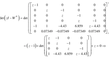
The eigenvalues of system can be obtained as:
1 0 0 0 0 0
0 1 0 0 0
0 0 1 0 0
det det
0 0 0 1 0
1 1 4.43 6.859 4.43 0
0 0.07349 0.07349 0.07349 0.07349 0
z z z zI W z z
1 0 0
0 1 0
1 det 0
0 0 1
1 4.43 6.859 4.43
1 0 0
0 1 0
det 1 det 0
0 0 1
1 4.43 6.859 4.43
z z
zI W z z
z z
1 0 0
0 1 0 2
det 1 0.524 1.91 0
0 0 1
1 4.43 6.859 4.43 1 1 1 2 0.524 3 1.9 4 z z
z z z
z z z z z z
This system is unstable.
In this step by applying feedback control law based on the Petri Nets model a controller is designed and consequently the system begins to be stabled. The following step should be taken to do so:
Step 1. The open loop poles of the system are calculated: 1 1 1 2 0.524 3 1.9 4 z z z z
Step 2. Define the desired pole locations with the characteristic equation.
4 3 2
0.2
0.525 0.7 0.8
0.775 0.423 0.249 0.059.
desired z
f z z z z
z z z z
Step 3. W+newK is constructed as follows:
1 0 0 0 0 0 0
0 0 1 0 0 0 0
0 0 0 1 0 0 0
0 1 2 3 4 0
0 0 0 0 1 0 0
1 1 4.43 6.859 4.43 0 1 0 0.07349 0.07349 0.07349 0.07349 0 0
newK
W k k k k
1 0 0 0 0 0
0 0 1 0 0 0
0 0 0 1 0 0
0 0 0 0 1 0
1 1 1 4.43 2 6.859 3 4.43 4 0 0 0.07349 0.07349 0.07349 0.07349 0
k k k k
1 0 0 0 0 0
0 0 1 0 0 0
0 0 0 1 0 0
0 0 0 0 1 0
1 1 1 4.43 2 6.859 3 4.43 4 0 0 0.07349 0.07349 0.07349 0.07349 0
newK
W
k k k k
The Petri Nets model with the feedback control law is shown in Fig. 6.
Step 4. The characteristic equation of W+newK is obtained as:
1 0 0 0 0 0
0 0 1 0 0 0
0 0 0 1 0 0
det det
0 0 0 0 1 0
1 1 1 4.43 2 6.859 3 4.43 4 0 0 0.07349 0.07349 0.07349 0.07349 0
0 1 0 0
0 0 1 0
1 det
0 0 0 1
1 1 4.43 2 6.859 3 4.43 4
zI WnewK
k k k k
z
k k k k
0
0 1 0 0
0 0 1 0
det 0
0 0 0 1
1 1 4.43 2 6.859 3 4.43 4
z
fnewk
k k k k
4 3 2
4 4.43 3 6.859 2 4.43 1 1 0
newk
Figure 6. Petri Nets modelling with feedback control law
Step 5. In this Step the following equation should be satisfied:
4 3 2
4 3 2 1
4 3 2
4.43 6.859 4.43 1
0.775 0.423 0.249 0.059
desired newk
newk desired
f z f z
f z z k z k z k z k
f z z z z z
Consequently, the K-vector is:
K=[k1 , k2 , k3 , k4]=[-0.941,4.18,-7.28,5.21]
This model has been simulated here. Fig. 7, shows the angle of the inverted pendulum step response without controller using Petri Nets model and state space model.
As it is shown above as the time increases, the deviation of pendulum angle increases too. Therefore, the system is unstable. The introduced Petri Nets method showed this fact clearly.
Figure 7. Step response of system with Petri Nets and state space model
Figure 8. Output of system with state space and Petri Nets approach controller
Fig. 8, illustrates the instable system with the feedback control law based on the state space model and Petri Nets approach, and it is obvious that after applying the controller, system begins to be stable.
By comparing responses in Fig. 8, it is shown that the Petri Nets model response is the same as the state space model. The comparative accuracy of this approach can be determined by investigating relative error. The output relative error between state space and Petri Nets approach controller is illustrated in Fig. 9.
0 10 20 30 40 50 60 70 80 90 100
-12 -10 -8 -6 -4 -2
0x 10
26
Sample
S
te
p
R
e
s
p
o
n
s
e
Petri Nets Model State Space Model
0 50 100
-0.2 -0.15 -0.1 -0.05 0 0.05 0.1 0.15
(a).Petri Nets Model
Sample (S)
s
te
p
R
e
s
p
o
n
s
e
0 50 100
-0.2 -0.15 -0.1 -0.05 0 0.05 0.1 0.15
(b).State Space Model
Sample (S)
s
te
p
R
e
s
p
o
n
s
Figure 9. Output error between state space and Petri Nets approach controller
The simulation results show that the dynamic behaviour including transient response, steady state response and steady state error is the same in both methods. Hence, the validity of the presented approach can be verified. The simulation of the
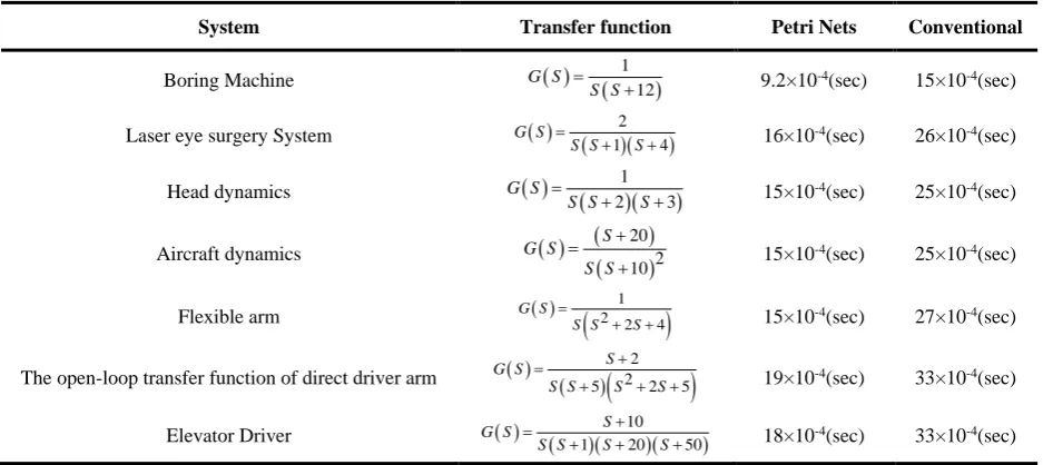
aforementioned system by our novel algorithm and the conventional one via the same hardware configuration relays a significant advantage of the new method which is the time efficiency. (The simulation time for the presented method was 0.0023 seconds compared to the 0.0063 seconds of the old one which means considerable amount of %64.27 decreases in run time). For further investigation, different types of common systems are considered and the time it takes to calculate the gains and simulate the model is compared [25]. Table 3 shows the simulation time result for the presented method compared to the conventional approach.
It can be observed that the advantage of the introduced method lies in reduced computation effort leading to time efficiency. Modelling with the Petri Nets provides powerful tools for the user. Petri Nets modelling gives graphical tools that provide an effective communication medium between the user and the system which enables us to model the dynamics of the systems visually.
Table 3. Simulation time results
System Transfer function Petri Nets Conventional
Boring Machine G S 112
S S
9.2×10⁻⁴(sec) 15×10-4(sec)
Laser eye surgery System G S 12 4
S S S
16×10-4(sec) 26×10-4(sec)
Head dynamics G S 21 3
S S S
15×10-4(sec) 25×10-4(sec)
Aircraft dynamics
20 2 10
S G S
S S
15×10-4(sec) 25×10-4(sec)
Flexible arm
1 2 2 4
G S
S S S
15×10-4(sec) 27×10-4(sec)
The open-loop transfer function of direct driver arm
2 25 2 5
S G S
S S S S
19×10-4(sec) 33×10-4(sec)
Elevator Driver G S 1S 1020 50
S S S S
18×10-4(sec) 33×10-4(sec)
6. Conclusion
A continuous system described by differential equations cannot be modelled by ordinary Continuous Petri Nets. To simplify modelling, controller design and analysis, this paper introduces Continuous -Time Delay- Petri Nets (CTDPN). CTDPN allows to model all continuous systems using simple rules. The principal equation of Petri Nets plays the same role as discrete state space equation. The properties of the discrete state space are reserved in incidence matrix. A simple algorithm for controller design by CTDPN based on state feedback control law is presented and
simulation results show this approach is effective and this method has much less complexities. By using CTDPN, a visual and systematic method for modelling the dynamics of a continuous system is presented which has considerably less run time compared to conventional approach. Besides, this method can be utilized to model hybrid systems with variable parameters or multiple subsystems which suggested for the further works on the basis of this approach.
0 10 20 30 40 50 60 70 80 90 100
-4 -3 -2 -1 0 1 2 3 4x 10
-15
Sample
R
e
la
ti
v
e
E
rr
o
References
[1] Z. Tao, L. Xie, D. Liang. Controller Design of DES Petri Nets with Mixed Constraint. Chinese Journal of Aeronautics, 2005, Vol. 18, No.3, 283- 288.
[2] M. Kloetzer, C. Mahulea, C. Belta, M. Silva. An Automated Framewor Formal Verification of Timed Continuous Petri Nets. IEEE Transactions on Industrial Informatics, 2010, Vol. 6, pp. 460-471. [3] K. Sacha. Fault Analysis Using Petri Nets. IEEE
Real-time Embedded Systems Workshop, 2001, pp. 130-133. [4] M. Durmus, S. Takai. Modeling Moving-Block
Railway Systems: A Generalized Batches Petri Net Approach. SICE Journal of Control, Measurementand SystemIntegration, 2013, Vol. 6, No. 6, 403–410. [5] E. Fesina, S. Savdur. Modeling of Sewage
Bioreme-diation as a Modified Petri Net. World Applied Scien-ces Journal, 2014, Vol. 31, No. 6, 1191-1197. [6] T. Jie, M. Ameedeen. A Survey of Petri Net Tools.
ARPN Journal of Engineering and Applied Sciences, 2014, Vol. 9, No. 8, 1209-1214.
[7] A. Dideban, M. Zareiee, H. Alla. Controller Syn-thesis with Very Simplified Linear Constraints in PN Model. 2nd IFAC Workshop on Dependable Control of Discrete Systems, Bari, Italy, 2009, pp. 265-270. [8] H. Alla, R. David. A Modeling and Analysis Tool for
Discrete Events Systems: Continuous Petri Net. Per-formance Evaluation, 1998, Vol. 33, No. 3, 175-199. [9] H. Apaydin-Ozkan, J. Julvez, C. Mahulea, M. Silva.
Approaching Minimum Time Control of Timed Continuous Petri Nets. Nonlinear Analysis: Hybrid Systems, 2011, Vol. 5, No. 2, 136-148.
[10] C. Vázquez, A. Ramírez-Treviño, M. Silva. Contro-llability of Timed Continuous Petri Nets with Uncontrollable Transitions. International Journal of Control, 2014, Vol. 87, No. 3, 537-552.
[11] Y. Wang, C. Chang. A Hierarchical Approach to Construct Petri Nets for Modeling the Fault Propagation Mechanisms in Sequential Operation. Computer & Chemical Engineering, 2003, Vol. 27, No. 2, 259-280.
[12] L. Recalde, E. Teruel, M. Silva. Autonomous Contin-uous P/T Systems. Lecture Notes in Computer Scien-ce: Application and Theory of Petri Nets, 20th Interna-tional Conference, USA, 1999, pp. 107–126.
[13] R. Champagnat, R. Valette, J. Hochon, H. Pingaud.
Modelling, Simulation and Analysis of Batch Produ-ction Systems. Discrete Event Dynamic Systems: Theo-ry and Applications, 2001, Vol. 11, No. 1, 119-136. [14] C. Vázquez, L. Recalde, M. Silva. Stochastic
Contin-uous-State Approximation of Markovian Petri Net Systems. 47th IEEE Conference on Decision and Cont-rol, Cancun, Mexico, 2008, pp. 901-906.
[15] D. Rowell. Analysis and Design of Feedback Control Systems: State-Space Representation of LTI Systems, 2002.
[16] A. Dideban, A. Ahangarani Farahani, M. Razavi.
Modeling Continuous Systems Using Modified Petri Nets Model. Modeling and Simulation in Electrical and Electronics Engineering (MSEEE), Semnan, Iran, 2015, Vol. 1, No. 2, pp. 75-79.
[17] A. Hartmann, F. Schreiber. Integrative Analysis of Metabolic Models–from Structure to Dynamics. Front Bioeng Biotechnol, 2015, Vol. 2, 1-10.
[18] Y. Q. Song, B. Li, K. Chen, T. Yang, H. Li. Relia-bility Research of the Traffic Signal System Based on
Extended Petri Nets. International Journal of Signal Processing, Image Processing and Pattern Recogni-tion, 2015, Vol. 8, 321-332.
[19] A. Dideban, M. Kiani, H. Alla. Implementation of Petri Nets Based Controller Using SFC. Journal of Control Engineering and Applied Informatics, 2011, Vol. 13, No. 4, 82-92.
[21] M. Alcaraz-Mejia, R. Campos-Rodriguez, E. Lopez-Mellado, A. Ramirez-Trevino. Partial Recon-figuration of Control Systems Using Petri Nets Struc-tural Redundancy. Information Technology and Con-trol, 2015, Vol. 44, No. 3, 287-301.
[22] E. Fraca, S. Haddad. Complexity Analysis of Conti-nuous Petri Nets. Fundamenta Informaticae, 2015, Vol. 137, 1-28.
[23] M. Kloetzer, C. Mahulea, C. Belta, L. Recalde, M. Silva. Formal Analysis of Timed Continuous Petri
Nets. In: 47th IEEE Conference on Decision and Control, Cancun, Mexico, 2008, pp. 245-250. [24] M. Sam Fadali. Digital Control Engineering: Analysis
and Design. Elsevier, USA, 2009.
[25] R. Dorf, R Bishop. Modern Control System. Prentice Hall, 9th Edition, 2011.