Advanced Spectral and Spatial Techniques for Hyperspectral Image Analysis and Classification

Advanced Spectral and Spatial Techniques

for Hyperspectral Image Analysis and

Classification

a dissertation presented by

Nicola Falco

in partial fulfilment of the requirements for the degree of

Doctor of Philosophy in the subject of

Information and Communication Technologies -Telecommunication Area

at the

Department of Information Engineering and Computer Science University of Trento

Trento, Italy

Electrical and Computer Engineering at the

Faculty of Electrical and Computer Engineering University of Iceland

Reykjavik, Iceland

Thesis Advisers:

Prof. Lorenzo Bruzzone

Prof. Jón Atli Benediktsson

Thesis Committee:

Prof. José M. Bioucas Dias

Prof. Gustau Camps-Valls

Advanced Spectral and Spatial Techniques for

Hyperspectral Image Analysis and Classification

Abstract

Recent advances in sensor technology have led to an increased availability of hyperspectral remote sensing images with high spectral and spatial resolu-tions. These images are composed by hundreds of contiguous spectral chan-nels, covering a wide spectral range of frequencies, in which each pixel contains a highly detailed representation of the reflectance of the materials present on the ground, and a better characterization in terms of geometrical detail. The burst of informative content conveyed in the hyperspectral images permits an improved characterization of different land coverages. In spite of that, it in-creases significantly the complexity of the analysis, introducing a series of chal-lenges that need to be addressed, such as the computational complexity and resources required.

This dissertation aims at defining novel strategies for the analysis and classi-fication of hyperspectral remote sensing images, placing the focal point on the investigation and optimisation techniques for the extraction and integration of spectral and spatial information. In the first part of the thesis, a thorough study on the analysis of the spectral information contained in the hyperspectral im-ages is presented. Though, independent component analysis (ICA) has been widely used to address several tasks in the remote sensing field, such as feature reduction, spectral unmixing and classification, its employment in extracting class-discriminant information remains a research topic open to further inves-tigation. To this extend, a profound study on the performances of different ICA algorithms is performed, highlighting their strengths and weaknesses in the hyperspectral image classification task. Based on this study, a novel ap-proach for feature reduction is proposed, where the use of ICA is optimised for the extraction of class-specific information. In the second part of the the-sis, the spatial information is exploited by employing operators from the math-ematical morphology framework. Morphological operators, such as attribute profiles and their multi-channel and multi-attribute extensions, are proved to be effective in the modelling of the spatial information, dealing, however, with issues such as the high feature dimensionality, the high intrinsic information redundancy and the a-priori need for parameter tuning in filtering, which are still open. Addressing the first two issues, the reduced attribute profiles are introduced, in this thesis, as an optimised version of the morphological

tribute profiles, with the property to compress all the meaningful geometrical information into a few features. Regarding the filter parameter tuning issue, an innovative strategy for automatic threshold selection is proposed. Inspired by the concept of granulometry, the proposed approach defines a novel gran-ulometric characteristic function, which provides information on the image decomposition according to a given measure. The approach exploits the tree representation of an image, allowing us to avoid additional filtering steps prior to the threshold selection, making the process computationally effective.

The outcome of this dissertation advances the state-of-the-art by proposing novel methodologies for accurate hyperspectral image classification, where the results obtained by extensive experimentation on various real hyperspectral data sets confirmed their effectiveness. Concluding the thesis, insightful and concrete remarks to the aforementioned issues are discussed.

Framsæknar aðferðir sem byggja á upplýsingum í rófi og

rúmi fyrir greiningu og flokkun mynda af mjög hárri vídd

Ágrip

Nýlegar framfarir í skynjaratækni hafa leitt til þess að nú er í meira mæli en áður hægt að afla fjarkönnunarmynda af afar hárri vídd (e. hyperspectral images) með mikilli upplausn, bæði í rófi og rúmi (e. spectral and spatial). Myndirnar eru samansettar af hundruðum samliggjandi rófrása sem ná yfir vítt tíðniróf og sérhver myndeining geymir í smáatriðum upplýsingar um endurkast efna sem eru á yfirborði jarðar auk nákvæmra upplýsinga um rúmfræðileg atriði. Hið mikla magn upplýsinga sem geymdar eru í myndum af hárri vídd leyfa betri framsetningu af þeim fjölbreytilegu gerðum landslags sem myndað er með fjarkönnunartækni. Þrátt fyrir þetta, er notkun á svona gögnum flókin í greiningu og huga þarf sérstaklega að ýmsum vandamálum, t.d. flóknari útreikningum og öflugum vélbúnaði sem þarf til úrvinnslunnar.

Í Þessari ritgerð er leitast við setja fram nýjar aðferðir til greiningar og flokku-nar fjarkönnuflokku-narmynda af mjög hárri vídd. Sérstök áhersla er lögð á rannsóknir og tækni við bestun til að draga fram róf- og rúmupplýsingar og þá síðan heil-dar upplýsingarnar. Í fyrri hluta ritgerðarinnar er kynnt ítarleg rannsókn á greiningu rófupplýsinga í fjarkönnunarmyndum af mjög hárri vídd. Þótt óháð þáttagreining (ICA – e. Independent Component Analysis) hafi víða verið no-tuð til að vinna ýmis verkefni í fjarkönnun, t.d. við víddarfækkun, afblöndun rófs og flokkun, þá er notkun ICA til að draga fram sundurgreiningarupplýsin-gar fyrir flokkun ekki vel þekkt og er hún enn viðfangsefni rannsókna. Af þes-sum sökum er hér gerð ítarleg rannsókn á frammistöðu nokkurra mismunandi ICA algríma, þar sem sérstaklega eru skoðaðir bæði styrkleikar og veikleikar algrímanna til flokkunar mynda af mjög hárri vídd. Í framhaldi af framangrein-dri rannsókn er ný víddarfækkunaraðferð sett fram. Í þessari aðferð er notkun ICA bestuð til að draga fram upplýsingar um einstaka flokka.

Í seinni hluta ritgerðarinnar eru rúmupplýsingar notaðar með upplýsingum sem fást með notkun virkja stærðfræðilegrar formfræði. Formfræðilegir virk-jar eins og auðkennaprófílar og útvíkkanir þeirra fyrir margar rásir og mörg auðkenni hafa reynst mjög öflugir til að gera líkön sem byggja á rúmfræði-legum upplýsingum. Hins vegar hefur reynst erfitt að leysa vandamál með þes-sari aðferð, þar sem fjöldi vídda verður oft mikill, umfremd (e. redundandcy) verður í gögnunum og nauðsynlegt er að skilgreina stika fyrirfram. Í ritgerðinni er unnið að lausn fyrstu tveggja vandamálanna.

Víddafækkun auðkennaprófíla er kynnt sem bestuð útgáfa formfræðilegra auðkennaprófíla með þeim eiginleika að öllum helstu flatarupplýsingum er þjappað inn í auðkenni. Þá er ný aðferð sem byggir á sjálfvirkri þröskuldun sett fram til að ákvarða síunarstika. Hún byggir á hugmyndinni um að nota sífellt stækkandi gildi á síunarstikum (e. granulometry), og er skilgreint sérstakt einkennisfall sem gefur upplýsingar um uppskiptingu myndarinnar samkvæmt gefinni mælingu. Nýja aðferðin notast við trjáframsetningu myndarinnar og losar okkur við viðbótarsíunarskref áður en valið á þröskuldunum fer fram. Það að losna við síunarskrefin gerir ferlið reiknilega hagkvæmt.

Niðurstöður þessarar ritgerðar eru framlag til stöðu þekkingar á fræðasviðinu þar sem kynntar eru nýjar aðferðir fyrir nákvæma flokkun

myndgagna af mjög hárri vídd. Niðurstöðurnar, sem fengust með

um-fangsmiklum tilraunum á margs konar raunverulegum gögnum af mjög hárri vídd, staðfestu gildi aðferðanna. Í lok ritgerðarinnar eru dregin saman og rædd atriði um framangreindar aðferðir og niðurstöður.

Acknowledgments

I would like to sincerely thank my advisers Jón Atli Benediktsson and Lorenzo Bruzzone, for their guidance, support, and most important, for their friend-ship, which gave me the possibility to learn and grow personally and profes-sionally during my doctoral studies.

I would like to thanks my colleagues at the VRII at Háskóli Íslands, Behnood, Eysteinn, Frosti, Gabriele, Pedram and Prashanth, for their friend-ship and support in the academic world and every-day life. A special thanks goes to Jakob for all the advices on my studies, the always interesting discus-sions, for helping in several occadiscus-sions, and most importantly, for letting me win at bowling. I wish to thank all the RSLab members at University of Trento, Ana-Maria, Begum, Claudia, Francesca, Davide, Leonardo, Massimo for shar-ing this experience and for all the time passed together. Special thanks go to Carlo and Sicong, for the reciprocal support during the research period.

I also wish to thank prof. José M. Bioucas Dias, prof. Gustau Camps-Valls and prof. Enrico Magli, for being part of the committee and for their comments and suggestions regarding the manuscript.

In these three years, I met many people and friends that made this period very special. A big thanks goes to Anna and Fabio, Atli Steinn, Gro, Hannes, Morgane, Pauline and Þorbjörg, for making my icelandic social life a bit more active. Going back to Italy, I must thanks my old friends Cippo, Enrico, Mitch, Mike, Preca, Simone, Toni for their company and for being always there when I was going back to Italy.

I want to thank Kyriaki, that with her enthusiasm and positivity gave me the strength to overtake any obstacle. Finally, a thought goes to my family, which has always been with me either when I was hundred or thousands miles far away from home, for supporting me and believing in me; this achievement would not have been possible without you.

Nicola February 2015

Contents

I Overview and Background

ljNj

1 Introduction 15

1.1 Overview on Remote Sensing . . . 15

1.2 Introduction to Hyperspectral Images . . . 17

1.3 Hyperspectral Image Classification: Challenges . . . 20

1.4 Objectives of this Dissertation . . . 22

1.5 Organization of the Dissertation . . . 24

2 Background and Related Work 25 2.1 Introduction . . . 25

2.2 Related Work . . . 26

2.2.1 Overview on Dimensionality Reduction Approaches 26 2.2.2 Overview on Spatial Information Extraction . . . . 29

2.3 Independent Component Analysis . . . 30

2.3.1 The Linear Mixing Model . . . 30

2.4 Morphological Operators . . . 32

2.4.1 Attribute Filters and Tree Representations . . . 33

2.4.2 Attribute Profiles . . . 34

2.4.3 Extension to Multi-Channel and Multi-Attribute . . 36

II Spectral Information Analysis

NjǏ

3.2 Independent Component Analysis (ICA) . . . 41

3.2.1 Infomax . . . 42

2 Contents

3.2.2 FastICA . . . 42

3.2.3 JADE . . . 44

3.2.4 RobustICA . . . 44

3.3 Design of Experiments and Investigations . . . 45

3.3.1 Experiment I: Low-Dimensional Space . . . 46

3.3.2 Experiment II: High-Dimensional Space . . . 47

3.3.3 Experiment III: Spatial Down-Sampling . . . 48

3.4 Experimental Setup . . . 48

3.4.1 ICA parameter tuning . . . 48

3.4.2 Feature Reduction . . . 49

3.4.3 Classification . . . 50

3.4.4 Data Sets’ Description . . . 51

3.5 Experimental Results and Discussion . . . 51

3.5.1 Experiment I: Low-Dimensional Space . . . 52

3.5.2 Experiment II: High-Dimensional Space . . . 57

3.5.3 Experiment III: Spatial Down-Sampling . . . 59

3.6 Conclusions . . . 66

4 Feature Reduction Based on ICA 69 4.1 Introduction . . . 69

4.2 Proposed Technique for Feature Reduction . . . 71

4.2.1 Extraction of Class-Specific ICs . . . 72

4.2.2 Evaluation of the Reconstruction Error . . . 72

4.2.3 Identification of the Optimal Mixing Matrix . . . 73

4.3 Experimental Setup . . . 74

4.3.1 FastICA Tuning . . . 74

4.3.2 Genetic Algorithm Tuning . . . 75

4.3.3 Classification . . . 75

4.3.4 Data Sets’ Description . . . 76

4.4 Experimental Results and Discussion . . . 76

4.5 Conclusions . . . 85

III

Integration of Spatial Information

ǐǏ

Contents 3

5.2.1 Attribute Profiles and Region Extraction . . . 91

5.2.2 Identification of the Representative Levels . . . 92

5.2.3 Fusion of the Attribute Profiles . . . 95

5.2.4 Extension to Multi-Channel and Multi-Attribute . . 95

5.3 Experimental Setup . . . 97

5.3.1 Classification . . . 98

5.4 Experimental Results and Discussion . . . 98

5.5 Conclusions . . . 99

6 Spectral and Spatial Information Integration 103 6.1 Introduction . . . 103

6.2 Design of Experiments and Investigations . . . 106

6.3 Experimental Setup . . . 106

6.3.1 Classification . . . 107

6.3.2 Data Sets’ Description . . . 107

6.4 Experimental Results and Discussion . . . 107

6.5 Conclusions . . . 111

7 Automatic Threshold Selection for Profiles 117 7.1 Introduction . . . 117

7.2 Proposed Automatic Threshold Selection . . . 119

7.2.1 Measure and Granulometric Characteristic Function 120 7.2.2 Threshold Selection . . . 121

7.3 Experimental Setup . . . 122

7.4 Experimental Results and Discussion . . . 122

7.5 Conclusions . . . 123

8 Conclusions 133 8.1 Contribution of this Dissertation . . . 134

8.2 Future Research Developments . . . 136

Appendix A Data Sets Description 139 A.1 Salinas Valley, California (Salinas) . . . 139

A.2 Hekla volcano, Iceland (Hekla) . . . 141

A.3 Okavango Delta, Botswana (Botswana) . . . 142

A.4 Pavia, university area, Italy (Pavia University) . . . 143

A.5 Pavia, central area, Italy (Pavia Center) . . . 144

4 Contents

A.6.1 AVIRIS . . . 146

A.6.2 Hyperion . . . 146

A.6.3 ROSIS-03 . . . 146

Appendix B Accuracy Assessment 147

List of Figures

1.1 Nadar élevant la Photographie à la hauteur de l’Art. . . 16

1.2 Comparison of the spatial and spectral sampling of the Land-sat TM and AVIRIS. . . 19

1.3 General scheme of a supervised image classification approach. 21

3.1 Experiment I: comparison of the overall classification accu-racy obtained by Infomax, FastICA and JADE for different DR strategies and different number of features. . . 53

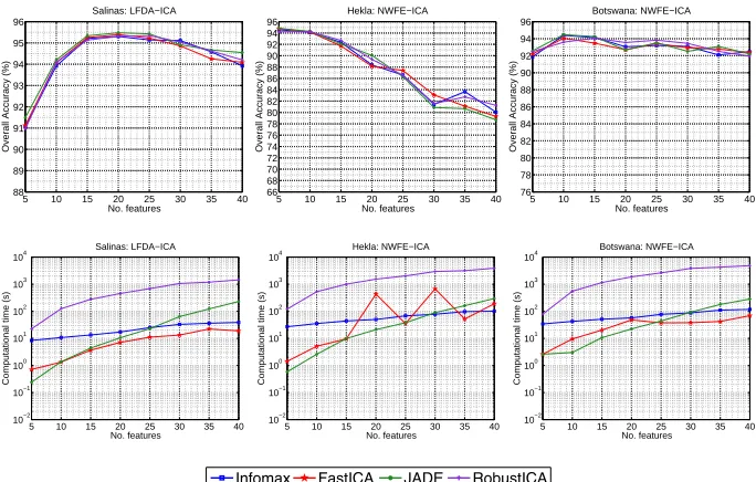
3.2 Experiment I: comparison of the overall classification accu-racy and computational cost obtained by Infomax, FastICA, JADE and RobustICA versus the number of features, consid-ering the best DR strategies. . . 56

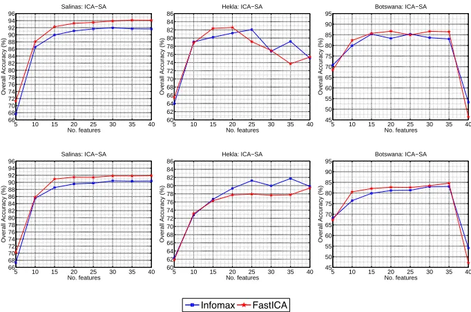
3.3 Experiment II: comparison of the overall classification accu-racy obtained by Infomax and FastICA versus the number of features by using SVM and RF. . . 58

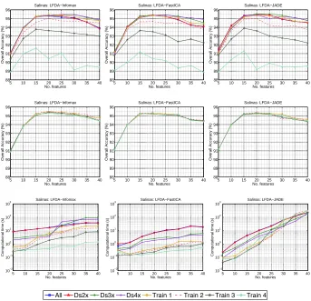
3.4 Experiment III in low dimensional scenario: comparison of the overall classification accuracy provided by Infomax, Fas-tICA and JADE, for different number of samples on Salinas data set. . . 61

3.5 Experiment III in low dimensional scenario: comparison of the overall classification accuracy provided by Infomax, Fas-tICA and JADE, for different number of samples on Hekla data set. . . 62

3.6 Experiment III in low dimensional scenario: comparison of the overall classification accuracy provided by Infomax, FastICA and JADE, for different number of samples on Botswana data set. . . 63

6 List of Figures

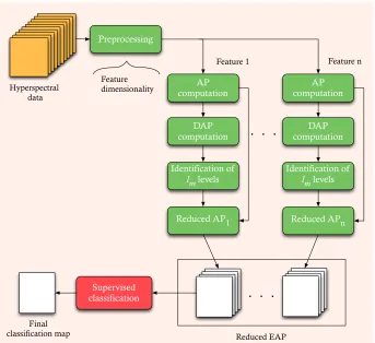
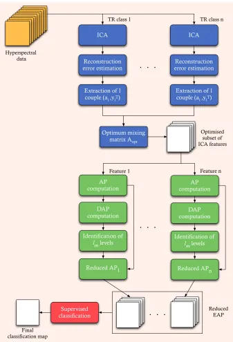
4.1 General scheme of the proposed technique for feature

reduc-tion based on ICA. . . 71

4.2 Clustering based on the training samples. . . 72

4.3 Selection based on genetic algorithm approach. . . 74

4.4 Subset of ICs extracted for Pavia University. . . 79

4.5 Subset of ICs extracted for Pavia Center. . . 80

4.6 Subset of ICs extracted for Salinas. . . 81

4.7 Subset of ICs extracted for Hekla. . . 82

4.8 Classification maps of Pavia University and Pavia Center . . 83

4.9 Classification maps of Salinas and Hekla . . . 84

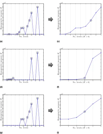
5.1 General scheme of the procedure to compute the reduce AP. 92 5.2 Examples of homogeneity measureH(C)for an increasing criterion. . . 94

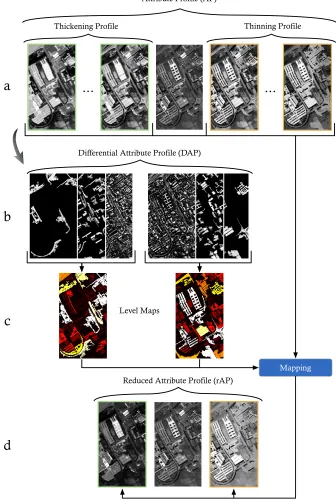
5.3 Pipeline of the processing required to obtain a reduced AP. . 96

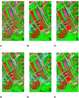
5.4 Classification maps of Pavia University by using: rEAPa; rEAPd; rEAPs; rEAPi; rEMAP. . . 101

6.1 General scheme of the proposed technique for spectral and spatial information integration for supervised classification. . 105

6.2 Classification maps of Pavia University: rEAPa; rEAPd; rEAPs; rEAPi; rEMAP. . . 112

6.3 Classification maps of Pavia Center: rEAPa; rEAPd; rEAPs; rEAPi; rEMAP. . . 113

6.4 Classification maps of Salinas: rEAPa; rEAPd; rEAPs; rEAPi; rEMAP. . . 114

6.5 Classification maps of Hekla: rEAPa; rEAPd; rEAPs; rEAPi; rEMAP. . . 115

7.1 General scheme for the proposed automatic threshold selec-tion technique. . . 119

7.2 Evaluation of the reconstruction error computed for the esti-mation of the GCFs derived by min-tree, max-tree and inclu-sion tree for Pavia University. . . 125

7.3 GCFs derived by min-tree, max-tree and inclusion tree, show-ing the breakpoints used to derived threshold. . . 126

7.4 Πφcomputed on Pavia based on GCFval. . . 127

7.5 Πφcomputed on Pavia based on GCFpix. . . 127

List of Figures 7

7.7 Πγcomputed on Pavia based on GCFval. . . 128

7.8 Πγcomputed on Pavia based on GCFpix. . . 129

7.9 Πγcomputed on Pavia based on GCFreg. . . 129

7.10 Πρcomputed on Pavia based on GCFval. . . 130

7.11 Πρcomputed on Pavia based on GCFpix. . . 130

7.12 Πρcomputed on Pavia based on GCFreg. . . 131

A.1 Salinas data set description. . . 140

A.2 Hekla data set description . . . 141

A.3 Botswana data set description . . . 142

A.4 Pavia University data set description . . . 144

List of Tables

1.1 Technical characteristics of some hyperspectral sensors de-veloped over last years [30]. . . 20

3.1 Classification results obtained in Experiment I (Figure3.1). Only the best results are reported. Classification results ob-tained on the original spectral channels are given for compar-ison. ”No. feat.” denotes the number of feature retained, ”OA (%)” denotes percentage overall accuracy, ”k” indicates the kappa coefficient and ”Time” gives the computational time in seconds. . . 55

3.2 Classification results obtained in Experiment I consider-ing RobustICA algorithm and the best DR strategies (Fig-ure3.2). Only the best results are reported. ”No. feat.” indi-cates the number of feature retained, ”OA (%)” denotes per-centage overall accuracy, ”k” gives the kappa coefficient and ”Time” gives the computational time in seconds. . . 57

3.3 Classification results obtained in Experiment II. Only the best results are reported. ”No. feat.” indicates the number of feature retained, ”OA (%)” denotes percentage overall ac-curacy, ”k” gives the kappa coefficient and ”Time” gives the computational time in seconds. . . 59

3.4 Experiment III: description of the data set considered in terms of numbers of samples. . . 60

3.5 Classification results obtained in Experiment III considering the high dimensional scenario. The results are related to Sali-nas data set by using FastICA. ”No. feat.” indicates the num-ber of feature retained, ”OA (%)” denotes percentage overall accuracy, ”k” gives the kappa coefficient and ”Time” gives the computational time in seconds. . . 64

10 List of Tables

4.1 Classification of the four data sets by employing the proposed ICA-based feature reduction approach. ”No. feat.” denotes the number of features selected based on the reconstruction error, ”No. feat. GA” denotes the number of features after the GA selection, ”OA (%)” indicates the percentage overall ac-curacies and ”k” indicates the kappa coefficients. Classifica-tion results obtained by exploiting the original spectral bands and by using the PCA-ICA strategy are given for comparison. 77

5.1 Comparison between the classification performance of the original EAPs and reduced EAPs for the Pavia University data set. For each attribute, the Table reports the percentage over-all accuracies ”OA(%)”, and the kappa coefficients ”k. Clas-sification results obtained by employing the original spectral bands and by using the four PCs exploited to built the EAP and rEAP are given for comparison. . . 98

6.1 Family of increasing criteria employed in Experiments 1 and 2 for each attribute. The number of thresholds is indicated in brackets. . . 106

6.2 Classification results obtained by exploiting the proposed technique for spectral and spatial classification. For each data set, the Table reports the percentage overall accuracies ”OA(%)” and the kappa coefficients ”k” obtained in Experi-ments 1 and 2 for each attribute. The number of features ex-ploited are given in parentheses. . . 108

6.3 Classification results obtained by exploiting the rEMAPs for Experiment 1 and 2. ”OA (%)” denotes the percentage over-all accuracies and ”k” indicates the kappa coefficients. . . 109

A.1 Classes and numbers of training / test samples for Salinas data set . . . 140

A.2 Classes and numbers of training / test samples for Hekla data set . . . 141

A.3 Classes and numbers of training / test samples for Botswana data set . . . 143

List of Tables 11

Part I

Overview and Background

1

Introduction

This Chapter introduces the dissertation, providing an overview on the re-mote sensing field, focusing on the hyperspectral images and the challenges related to their analysis. The objectives and the contributions are then de-scribed.

1.1 Overview on Remote Sensing

The innate human desire to explore and understand the intangible pushes the boundaries of the scientific and technical limits, and is what made remote sens-ing the field of science of today. Aristotle, in De Anima, exposes the nature of light as a state of actual transparency in a potentially transparent medium and thus represents the necessary condition for vision. Eighteen hundred years after him, Leonardo da Vinci sets in detail the principles underlying the “cam-era obscura”, while Isaac Newton, in 1666, using a prism proves that the light could be dispersed into a spectrum of colours, and using a second prism, the color could be re-combined into white light, giving birth to the science and art of “drawing with light”, broadly known as “photography”. Not long after, the first photograph in history of humanity was taken by Niepce (1827), while Gaspard-Félix Tournachon (Nadar) took in 1858 the first aerial photograph from a balloon from an altitude of 1,200 feet over Paris. New methods and

16 1. Introduction

technologies for sensing of the Earth’s surface going beyond the traditional black and white aerial photograph, required a new, more comprehensive term to be established. The termremote sensingcame to fill in this gap, initially in-troduced in 1960. Remote Sensing(RS) is the field of science that includes all those activities necessary for the observation, acquisition and interpreta-tion of informainterpreta-tion related to objects, events, phenomena or any other item under investigation, without making physical contact with the object, event, or phenomenon under investigation. Since the launch of the first satellite for space exploration (Sputnik-1) in the late fifties, advances in the satellite tech-nology burst, offering a multitude of spaceborne and airborne platforms with on-board sensors able to detect a great number of heterogeneous sources of information, for the study not only of distant celestial objects but also for the Earth Observation (EO).

Figure 1.1: Honoré Daumier (French, 1808-1879). Nadar Élevant la Pho-tographie à la Hauteur de l’Art, May 25, 1862. Brooklyn Museum photo-graph, 2004.

Remote sensing systems collect data by de-tecting the energy that is reflected from an ob-ject or area under investigation. Considering the electromagnetic radiation as the principal physical carrier of information, a main differ-entiation of remote sensing systems is based on the typology of the source of energy exploited. Depending on whether these systems measure the radiation that is naturally available, or the energy used to illuminate the target under in-vestigation is emitted by the sensor, are defined as passive or active, respectively. Passive sen-sors rely on the energy provided by the Sun, which is either reflected, or absorbed and then re-emitted from the Earth’s surface. While the reflected energy (e.g., visible radiation) is

1.2. Introduction to Hyperspectral Images 17

The vast variety of available sensors, which provide data either in image or signal formats, allows to tackle a large number of applications with remark-able advantages. In general, each family of sensors is characterised by prop-erties such as spatial, spectral, radiometrical and temporal resolutions, which are strictly related to their physical implementation resulting more or less suit-able for a precise application. This entails the development of advanced tech-niques for data processing and interpretation that are sensor and application dependent. Space exploration is the RS domain that leads by far the techno-logical advances, providing important know-how also for the Earth monitoring and for its understanding as a celestial object. Another main application is re-lated to the environmental monitoring, where remote sensing techniques are used for studying human activities, such as urban planning, agriculture land us-age, and natural phenomena, such as damage assessment due to earthquakes or floods, eruptions, climate change (e.g. glaciers), deforestation. Protected areas with fragile ecosystems can be studied by means of non-invasive remote sensing-based monitoring, without carrying any risk of environmental dam-age, replacing in this way costly field campaigns. Other important applications include meteorology, national security and natural resource management. The dissemination of remote sensing data is another important topic and is strictly connected to geographic information systems (GIS). Such platform allows re-mote sensing data obtained by different sources to be combined in order to make the information readily understandable to the final users.

1.2 Introduction to Hyperspectral Images

Earth remote sensing includes data collection on the environment, geology, climate, and other characteristics of the Earth by means of sensors positioned in the air or in Earth orbit. An important distinction between the systems broadly used to this end, refers to the coverage of electromagnetic spectrum. Focusing on passive optical systems, the sensor acquires data as in image for-mat, detecting a portion of the electromagnetic radiation reflected from the Earth’s surface in a range of wavelengths that includes the visible, near-infrared and short-wavelength infrared regions of the electromagnetic spectrum.

18 1. Introduction

of spectral filters and optical components (e.g., prism, grating). For a more detailed review on sensor systems and different typology of scanners, please refer to [87,91,92]. According to the characteristics of the scanner, sensor systems are distinguished by their different resolutions, which also define the characteristics of the acquired images. The minimum size of an object that the sensor is able to distinguish from the ground represents the spatial resolution, and depends on the altitude of the sensor and its angle of view (i.e., the an-gle subtended by the sensor), which is defined in terms of Instantaneous Field Of View (IFOV). In digital imaging, the resolution is limited by the pixel size. The spectral resolution is the minimum wavelength at which the instrument is sensitive, while the radiometric resolution is defined as the minimum energy able to be detected by the sensing system. The intrinsic radiometric resolu-tion of a sensor depends on the detector’s signal to noise ratio. In a digital image, the radiometric resolution is limited by the number of discrete quan-tisation levels used to digitise the continuous intensity value. Considering a three-dimensional space (x, y, λ), wherexandyare spatial coordinates andλ

1.2. Introduction to Hyperspectral Images 19

1.4 Remote-Sensing Systems 19

The grid of pixels that constitutes a digital image is achieved by a combination of scanning in the cross-track direction (orthogonal to the motion of the sensor platform) and by the platform motion along the in-track direction (Fig. 1-10) (Slater, 1980). A pixel is created whenever the sen-sor system electronically samples the continuous data stream provided by the scanning. A line scanner uses a single detector element to scan the entire scene. Whiskbroom scanners, such as the Landsat TM, use several detector elements, aligned in-track, to achieve parallel scanning during each cycle of the scan mirror. A related type of scanner is the paddlebroom, exemplified by AVHRR and MODIS, with a two-sided mirror that rotates 360°, scanning continuously cross-track. A signif-icant difference between paddlebroom and whiskbroom scanners is that the paddlebroom always scans in the same direction, while the whiskbroom reverses direction for each scan. Pushbroom scanners, such as SPOT, have a linear array of thousands of detector elements, aligned cross-track, which scan the full width of the collected data in parallel as the platform moves. For all types of scanners, the full cross-track angular coverage is called the Field Of View (FOV) and the corre-sponding ground coverage is called the Ground-projected Field Of View (GFOV).9

FIGURE 1-9. Comparison of the spatial and spectral sampling of the Landsat TM and AVIRIS in the VNIR spectral range. Each small rectangular box represents the spatial-spectral integration region of one image pixel. The TM samples the spectral dimension incompletely and with relatively broad spectral bands, while AVIRIS has relatively continuous spectral sampling over the VNIR range. AVIRIS also has a somewhat smaller GSI (20m) compared to TM (30m). This type of volume visualization for spatial-spectral image data is called an “image cube” (Sect. 9.9.1).

9. Also called the swath width, or sometimes, the footprint of the sensor. 1 2 3

4 band 400 900 wavelength (nm) x λ TM y 400 900 wavelength (nm) 1 band 50 AVIRIS

Figure 1.2:Comparison of the spatial and spectral sampling of the Landsat TM and AVIRIS in the VNIR spectral range. Each cell represents the spatial-spectral integration region of one pixel. The sampling of the spectral dimension operated by the Landsat TM results incomplete with relatively broad spectral bands, while the spectral sampling in the case of AVIRIS is relatively continuous over the VNIR range [92].

20 1. Introduction

Table 1.1:Technical characteristics of some hyperspectral sensors developed over last years [30].

Sensor Manufacturer Platform No. of Spectral Spectral

bands resolution range

Hyperion NASA GSFC Satellite 220 10nm 0.4-2.5 μm

MODIS NASA Satellite 36 40nm 0.4-14.3 μm

CHRIS Proba ESA Satellite up to 63 1.25nm 0.415-1.05 μm

AVIRIS NASA JPL Aerial 224 10nm 0.4-2.5 μm

HYDICE Naval Research Lab Aerial 210 7.6nm 0.4-2.5 μm

PROBE-1 Earth Search Science Aerial 128 12nm 0.4-2.45 μm

CASI 550 ITRES Research Ltd Aerial 288 1.9nm 0.4-1 μm

CASI 1500 ITRES Research Ltd Aerial 288 2.5nm 0.4-1.05 μm

SASI 600 ITRES Research Ltd Aerial 100 15nm 0.95-2.45 μm

TASI 600 ITRES Research Ltd Aerial 64 250nm 8-11.5 μm

HyMap Intergrated Spectronics Aerial 125 17nm 0.4-2.5 μm

ROSIS-3 DLR Aerial 115 4nm 0.43-0.85 μm

EPS-H GER Corporation Aerial 133 0.67nm 0.43-12.5 μm

EPS-A GER Corporation Aerial 31 23nm 0.43-12.5 μm

DAIS 7915 GER Corporation Aerial 79 15nm 0.43-12.3 μm

AISA Eagle Spectral Imaging Aerial 244 2.3nm 0.4-0.97 μm

AISA Eaglet Spectral Imaging Aerial 200 - 0.4-1.0 μm

AISA Hawk Spectral Imaging Aerial 320 8.5nm 0.97-2.45 μm

AISA Dual Spectral Imaging Aerial 500 2.9nm 0.4-2.45 μm

MIVIS Daedalus Aerial 102 20nm 0.43-12.7 μm

AVNIR OKSI Aerial 60 10nm 0.43-1.03 μm

properties, hyperspectral images have been widely exploited in different appli-cations, ranging from forestry management, pollution detection and mineral exploration. Table1.1provides a summary of the most commonly used sen-sors usually mounted on aircraft or spacecraft, reporting the principal spectral characteristics.

1.3 Hyperspectral Image Classification: Challenges

1.3. Hyperspectral Image Classification: Challenges 21

Data Processing

Prior information

Hyperspectral data

Final classification map

Classification

Supervised classification

Figure 1.3:General scheme of a supervised image classification approach. Available prior information can be used in both the classification stage and the data processing stage.

into the so-called “classes” of coverage present on the ground of the investi-gated area of interest. Product of this process is a thematic map, where pixels are characterised by a given label, usually represented by a colour or symbol, used to uniquely identify the items within a class. A general scheme of image classification is illustrated in Figure1.3, in which available information can be exploited in both the data processing and the classification stage. If on the one hand the burst of informative content conveyed in hyperspectral images, rep-resented by both high spectral and spatial resolutions, provides the base for obtaining high accuracy in the identification of different land-covers, on the other hand it introduces a number of challenges that need to be efficiently ad-dressed.

22 1. Introduction

In the machine learning domain, this behaviour is known as the Hughes phe-nomenon (named after Gordon F. Hughes) [54].

Second, the increase of the spatial resolution in the new generation of spec-trometers introduces other important issues in the analysis and classification of hyperspectral images. The high geometrical detail of the scene leads to the presence of objects that are composed by several spatial correlated pixels, re-sulting in an increase of the intraclass variability [13]. The aforementioned phenomenon decreases the effectiveness of the analysis when only the spec-tral information is considered, enforcing the need of strategies that integrate the analysis of both spectral and contextual domains in order to maximize the exploitation of the information combined in these images.

1.4 Objectives of this Dissertation

The research work presented in this dissertation aims at investigating and defining novel techniques for the analysis and supervised classification of re-mote sensing hyperspectral images. In particular, the focus is on the investi-gation and optimisation of strategies, based on the use of independent com-ponent analysis (ICA) and morphological operators, for the extraction and integration of both spectral and spatial information contained in hyperspec-tral images. In recent studies, ICA proved its effectiveness in extracting useful information to address the hyperspectral image classification task. However, many issues related to the computational cost and how to effectively extract class-specific information, need to be further investigated. Morphological op-erators, such as morphological attribute profiles and their multi-channel and multi-attribute extensions, proved to be effective in modelling the spatial char-acteristics. However, issues such as parameter tuning in filtering, need to be addressed, in order to obtain a reliable and representative image decomposi-tion. The high dimensionality of the profiles, which leads to a high intrinsic information redundancy and thus to the Hughes phenomenon, is still an open issue.

Aiming at overcoming the aforementioned issues and limitations that affect the analysis of hyperspectral image classification, the following objectives are defined:

1.4. Objectives of this Dissertation 23

different experimental set-ups.

• to develop a novel strategies to limit the Hughes phenomenon for hy-perspectral image classification by exploiting ICA.

• to design an innovative technique for spatial information extraction by using morphological attribute profiles, while addressing the informa-tion redundancy issue.

• to move towards a fully automatic approach to the selection of filtering parameters used for the computation of attribute profiles.

24 1. Introduction

1.5 Organization of the Dissertation

This dissertation is organised as follows:

Part I provides an introduction to the remote sensing field and the context in which the dissertation is developed.

Chapter1introduces the remote sensing field, providing a description of both the challenges and the objectives addressed in this thesis.

Chapter2presents an overview of the state-of-the-art in spatial and spectral information extraction domains. Moreover, it provides the theoretical back-ground on independent component analysis and morphological operators.

Part II includes the strategies developed for spectral information extraction based on the exploitation of ICA.

Chapter3presents a thorough study on the performances of different indepen-dent component analysis algorithms for the extraction of class-discriminant information in remote sensing hyperspectral image classification.

Chapter4describes a novel feature reduction technique based on ICA, whose aim is to extract subsets of class-specific independent components for the hyperspectral image classification.

Part III presents the contributions of this dissertation on spectral-spatial analysis for hyperspectral image classification.

Chapter 5 introduces the novel concept of reduced attribute profiles as an optimised version of the morphological attribute profiles. This Chapter provides a solution to both the high dimensionality and the information redundancy issues that affect the morphological attribute profiles.

Chapter 6 presents a new methodology that combines the findings in Chapter 4 and Chapter 5, fusing the spectral and spatial information for hyperspectral image classification.

Chapter7introduces a step towards a fully automated procedure for building the attribute profiles, presenting a novel automatic strategy for threshold selection.

2

Background and Related Work

This Chapter provides an overview on the most widely used spectral and spatial techniques developed over the last years in pattern recognition, ma-chine learning and image processing, for the analysis of hyperspectral im-ages. Then, the theoretical background on both independent component analysis and morphological operators is provided.

2.1 Introduction

Image classification in hyperspectral remote sensing images is a complex task that employs a number of processes aiming at addressing the challenging is-sues that emerge from the nature of the hyperspectral images. Considering the spectral domain, each single pixel is considered as an independent entity of information. The high dimensionality makes the analysis computationally ex-pensive, while the Hughes’ phenomenon (curse of dimensionality) [54] arises when the ratio between the number of available training samples and the num-ber of spectral channels is small. This affects the generalization capability of the classifier. Most studies in the current literature address the curse of di-mensionality issue by exploiting feature extraction and feature selection tech-niques, aiming at decreasing the dimensionality of the feature space by retain-ing the most useful information. Other issues arise when hyperspectral images

26 2. Background and Related Work

with improved spatial resolution, where the scene is characterized by objects composed by groups of pixels highly correlated, are considered. The improved detail increases the complexity of the image, adding a certain spectral variabil-ity to the pixels that belong to the same object or class The complexvariabil-ity increases by increasing of the spatial resolution. In this context, approaches based only the spectral information result less effective, providing classification maps with high uncertainty, especially for those classes with limited number of samples. Therefore, in order to minimise the uncertainty of the classification, the con-textual information should be extracted and included in the analysis. In this Chapter, an overview of the most widely used techniques for dimensionality reduction and spatial information extraction approaches is presented, focusing on independent component analysis and mathematical morphology, which are the techniques that will be considered in this dissertation.

2.2 Related Work

2.2.1 Overview on Dimensionality Reduction Approaches

High-dimensional data sets present many mathematical challenges as well as some opportunities, and are bound to give rise to new theoretical develop-ments. One of the problems with high-dimensional datasets is that, in many cases, not all the measured variables are “important” for understanding the un-derlying phenomena of interest. Dimensionality reduction can be seen as the process of deriving a set of degrees of freedom, which can be used to repro-duce most of the variability of a data set. Dimensionality reduction has a long history as an approach to data visualisation, and for extracting key low dimen-sional features. Apart from teaching us about the data, dimendimen-sionality reduc-tion can lead us to better models for inference. It can be divided into two major components, the feature selection and the feature extraction.

2.2. Related Work 27

spectral channels) an exhaustive search strategy would result to be not feasible from the computational perspective. Sub-optimal strategies are broadly used, such as the Sequential Backward Selection (SBS) [71] and the Sequential For-ward Selection (SFS) [107] methods. The first method performs a top-down search where the final feature subset is built up by starting from the complete set of features, while the second method applies a bottom-up search strategy, in which the starting point is an empty set. Both the methods are affected by the so-called nesting effect [58,86]. In case of SBS technique, the discarded fea-tures cannot be selected again and added to the subset while in the case of SFS the selected features cannot be discarded in a second moment. The Sequential Forward Floating Selection (SFFS) and the Sequential Backward Floating Se-lection (SBFS) [86] methods were proposed to overcome the nesting effect. The steepest ascent and the fast constrained [93] algorithms, in which the fea-ture selection problem is represented by a multi-dimensional binary space, are effective strategies that have shown better results compared to SFFS technique, even if the required computation time is slightly higher. Furthermore, heuris-tic search algorithms based on the evolutionary concept of natural selection, such as Genetic Algorithms (GAs) [46], are also used in several fields as well as in hyperspectral image analysis, where multi-objective fitness function can be used to find useful spatially invariant features for image classification [14].

num-28 2. Background and Related Work

ber of training samples for a high-dimensional space, since the computation of the class-statistical parameters is performed at full dimensionality. Con-sidering the case of a limited number of training samples, Projection Pursuit (PP) [59] was proposed in order to avoid the computation at full dimension-ality, which is done in a lower-dimensional subspace. The method achieves the dimensionality reduction by optimizing a projection index, which is the minimum Bhattacharyya distance among the classes, taking into considera-tion first-order and second-order statistics. Non-parametric Weighted Feature Extraction (NWFE) [63] was proposed as a trade-off between the advantages and limitations of the DAFE and DBFE techniques. The method weights every sample to compute the local means and defines new non-parametric between-class and within-between-class scatter matrices to get more features. However, these techniques are affected by a higher computational load, making the all feature extraction process considerably slow.

2.2. Related Work 29

2.2.2 Overview on Spatial Information Extraction

30 2. Background and Related Work

the geometrical detail of the unfiltered regions is fully preserved. This high flexibility renders the APs a powerful tool for extracting complementary spa-tial information of the structures in the scene.

2.3 Independent Component Analysis

The high dimensionality of hyperspectral data can provide a better character-ization of the spectral behaviour of different land-covers, however the redun-dancy of information should be detected and discarded in order to improve the discriminant analysis. In general, in pre-processing steps, a PCA transfor-mation is applied to the data in order to reduce the dimensionality and obtain a better representation of the whole dataset with a smaller signal to noise ra-tio. Due to the nature of this orthogonal transformation, the approach results to be not class discriminant, obtaining a new feature space in which, usually, only the first few components are considered, neglecting possible information. Moreover, in the case of non-Gaussian processes, as the class distributions are in hyperspectral data, the variance may not be the quantity of interest. Based on higher order statistics, ICA could be used as a feature extraction approach for extracting the most representative components from hyperspectal images. ICA is a well known unsupervised blind source separation technique, ex-tensively used in several fields, aimed at finding statistically independent com-ponents (ICs) by only considering the observation of mixture signals. The problem of blind separation has been widely investigated in various field such as biomedical signal analysis and processing, e.g., in electroencephalog-raphy (EEG), in electrocardiogelectroencephalog-raphy (ECG), in electromyogelectroencephalog-raphy (EMG), in magnetoencephalography (MEG) and in electronystagmography (ENG) [60,70, 82, 98,104]. ICA-based methods are also applied to geophysical data processing, data mining, speech enhancement, image recognition and wireless communications [23]. During the most recent years, ICA has also received attention in the hyperspectral remote sensing data analysis, in par-ticular for feature reduction [106], spatial unmixing [79], and classification [29,32,81,105].

2.3.1 The Linear Mixing Model

2.3. Independent Component Analysis 31

model can be written as:

xi =ai,1s1+ai,2s2+...+ai,nsn i=1, ...,n. (2.1) In terms of random vectors, the model can be rewritten as:

x = As, (2.2)

wherex = [x1,x2, ...,xn]T is the observed vector, A is the unknown mix-ing matrix with elementaij,i,j = 1, ...,n(which are real coefficients) and s= [s1,s2, ...,sn]Tis the unknown source vector. By estimating the unmixing matrix ofA, calledW, thesvector that represents the independent compo-nents (ICs) is obtained by:

s = Wx. (2.3)

The estimation of the ICA model is possible if the following assumptions and restrictions are satisfied: 1) the sources are statistically independent; 2) the independent components must have a non-Gaussian distribution; 3) the un-known mixing matrixAis assumed square and full rank. Under these condi-tions, the ICA model can be rewritten as:

y =Wx ≃s, (2.4)

whereW≃A−1_{. The problem can be solved by estimatingWto obtainythat}

represents the best possible approximation ofs. Nevertheless, sinceWands are unknown in the ICA model, three ambiguities necessarily hold:

1. The variances (energies) of the independent components cannot be de-termined. That is because any scalar multiplier in one of the sourcessi could always be canceled by dividing the corresponding columnaiofA by the same scalar.

2. For similar reasons, also the order of the independent components can-not be ranked.

3. The sign cannot be determined. This means that dark and bright regions may have the same meaning, which is not critical in most applications.

defini-32 2. Background and Related Work

tion of these algorithms will be provided in Chapter3, where a detailed com-parison among them is presented.

2.4 Morphological Operators

2.4. Morphological Operators 33

is not shape-dependent any more, whereas, it is adaptive to the considered re-gion and its surrounding. In a similar ways as for the morphological filters, it is possible for the attribute filters to build a multi-scale representation of the images, i.e., morphological attribute profiles (APs) [26].

2.4.1 Attribute Filters and Tree Representations

A two-dimensional gray-scale imageI, which can be defined as a mapping from the image domainE ⊆intoZ, can be fully represented as a set of connected componentsC, defining a partitionπiofE. The wayCis defined leads to differ-ent partitions. If we consider a connected operatorψ, by definition it will op-erate onIonly by merging the connected components of the given setC[88]. Thus, the result of the filtering will be a new partitionπψthat is coarser (i.e., containing less regions) than the initial one, meaning that for each pixelp ∈E,

πI(p)⊆ πψ(I)(p)[78, Chapter 7]. The coarseness of the partition generated by

a connected operator is determined by a parameterλ(i.e., a size-related filter parameter). Given two instances of the same connected operator with differ-ent filtering parameters,ψ_λiandψ_λj, which we denote for simplicity asψ_iand

ψ_j, respectively, there is an ordering relation between the resulting partitions:

πψ_i ⊆ πψ_j givenλi ≤ λj. Among the different types of connected operators, attribute filters (AFs) are largely diffused. AFs filter connected components in Caccording to an attributeAthat is computed on each component. In partic-ular, the value of an attributeAis evaluated on each connected component in Cand this measure is compared with a reference thresholdλin a binary pred-icateTλ(e.g.,Tλ := A ≥ λ). In general terms, if the predicate is true the component is maintained otherwise it is removed. According to the attribute considered, different filtering effects can be obtained leading to a simplification of the image. These effects are driven by characteristics such as the regions’ scale, shape or contrast. Indeed, the high flexibility of the attribute filter relies on their capability in modelling the spatial information based on any measure that could be computed on a connected component, ranging from measures that are purely geometric (e.g. area, length of the perimeter, image moments, shape factors), to textural ones (e.g. range, standard deviation, entropy), and more.

34 2. Background and Related Work

the tree data representation is able to increase the filtering efficiency. In the first phase, the tree structure is created, where the connected components are identified and the hierarchical structure between nodes is defined. In the sec-ond phase, the criterion is evaluated at each node, preserving the nodes that satisfy a given binary predicateT, and removing the others. The final phase is the image restitution, where the pruned tree is converted back to the im-age. Attribute filters are among those filters that can be easily implemented on tree representations since they natively work on connected components (con-versely to connected filters based on structuring elements). According to the way the set of connected componentsC is defined, different tree representa-tions of the same image and hence different filters are obtained. A max-tree

representation is obtained by considering the upper level setU(f) = {X :

X ∈ C([f ≥ λ]),λ ∈ Z}. By pruning the max-tree, an anti-extensive filter is obtained (i.e., bright regions will be removed), thus, if the operator is also idempotent and increasing, it leads to an opening. Analogously, amin-tree rep-resentation and an attribute closing operator are obtained by considering the lower level setL(_f) ={_X :_X∈ C([_f ≤ _λ]),_λ ∈Z}_{, in which the connected} components are defined according to a decreasing ordering relation. A differ-ent tree represdiffer-entation is given by theinclusion tree(ortree of shapes) in which the components are defined by a saturation operator that fills holes in compo-nents. A hole in a regionX ∈ Cis defined as a component that is completely surrounded byX. The inclusion tree is constructed by progressively saturating the image starting from its regional extrema (i.e., local maxima and minima in the image) until reaching only a single component fully coveringE. The inclu-sion tree can equivalently be obtained by merging the upper and the lower level sets of an image [17]. The sequence of inclusions induced by saturation deter-mines the components in the tree and their links defining the hierarchy. Since the saturation operator is contrast invariant (i.e., bright and dark regions will be treated the same), the filters operating on this tree will be self-dual (quasi self-dual in the case of discrete images).

2.4.2 Attribute Profiles

LetIbe a digital grey-scale image andZn(n=_{2, i.e., 2D images) its definition}

domain. A morphological transformation,ψ, is a mapping from a subset,E, of the image domain,I, to the same definition domain,E, withψ(I)→Zn_{. A} pro-file Π(_I)_{is defines as a sequential filtering performed by considering a family}

2.4. Morphological Operators 35

λis a set of reference scalar values used in the filtering andCis a connected region in the image. Following this definition and considering a max- and a min-tree, the attribute opening profile, ΠγT, and the attribute closing profile, ΠφT, can be defined as follows:

ΠγT(I) =

{

ΠγTλ :ΠγTλ =γTλ(I), ∀λ∈[0, ...,L]

}

(2.5)

ΠφT(I) =

{

ΠφTλ :ΠφTλ =φTλ(I), ∀λ∈[0, ...,L]

}

, (2.6)

whereφTλ andγTλrepresent a morphological attribute closing and attribute opening, respectively. The attribute profile, Π(I), is obtained by concatenating the opening and closing profiles as follows:

Π(I) = {

Π−_φT(I),I,ΠγT(I)

}

, (2.7)

whereI = _ΠφT₀ = ΠγT₀ correspond to the original grey-scaleI, and Π− φT(I) represents the ΠφT(I)in reverse order. It can be seen that the profile results in a vector of 2L+1 images.

Another important operator that is extensively used in this work is the so-called differential attribute profiles (DAP), Δ(I). It is obtained by computing the derivative of the AP, and it shows the residual of the progressive filtering, i.e., the connected regions that have been filtered between two adjacent levels of the AP, and their relative grey values. The DAP can be defined as follows:

Δ(I) = {ΔφT(I),ΔγT(I)

}

. (2.8)

In this case, the obtained profile is represented by a vector of 2limages. A con-cept that worth mentioning is the possibility to have non-increasing criteria, which leads to more general definitions of opening and closing, withφTλ_and

γTλdenoting the thickening and the thinning profiles, respectively.

Analogously, when considering the contrast invariant operatorρ, which is based on the inclusion tree, the profile Πρ, named self-dual attribute profile (SDAP) [18,28], can be obtained:

Πρ(I) = {

ΠρTλ :ΠρTλ =ρTλ(I), ∀λ∈[0, ...,L]

}

(2.9)

36 2. Background and Related Work

2.4.3 Extension to Multi-Channel and Multi-Attribute

Morphological operators are in general non-linear connected transformations computed on an ordered set of values. This means that any their extension to multivariate values is an ill-posed problem. The usual strategy is to apply the operator to each channel separately and fuse or create a stack of the obtained profiles. However, in the case of hyperspectral images, which feature space has a high dimensionality, this strategy becomes unattainable. In [7], a mor-phological operator was applied to a sub-space of the original data obtained by using PCA, and only the first most informative principal components (PCs) were considered. The concatenation of each obtained MPs resulted in a new structure, called extended morphological profile (EMP).

Analogously, the same procedure can be adopted for the APs case [27] and SDAP. LetIbe a multi-channel data composed ofrfeatures. The extended morphological attribute profiles (EAP) is defined as the concatenation of the AP built on each featuref:

EAP(_I) = {

Π(_f1),_Π(_f2), ...,_Π(_fr) }

. _(2.10)

A further extension, which is based on the flexibility of the AP in considering any possible measure applicable to a connected region as criterion, is the con-catenation of the EAPs obtained by different attributes, which results in the definition of the extended multi-attribute profile (EMAP) [27]:

EMAP(I) = {

EAP(I)_a1,EAP(I)_a2, ...,EAP(I)_aq }

, (2.11)

Part II

Spectral Information Analysis

3

Analysis of ICA Algorithms

This Chapter presents a thorough study on the performances of different Independent Component Analysis (ICA) algorithms for the extraction of class-discriminant information in remote sensing hyperspectral image classification. The analysis aims to address a number of important issues regarding the use of ICA in the RS domain. Three scenarios are consid-ered and the performances of the ICA algorithms are evaluated and com-pared against each other, in order to reach the final goal of identifying the most suitable approach to the analysis of hyperspectral images in super-vised classification.

3.1 Introduction

ICA is a well known unsupervised blind source separation technique, exten-sively used in several fields, aimed at finding statistically independent compo-nents (ICs) by only considering the observation of mixture signals. When ap-plied to hyperspectral data, ICA extracts the source components that generate the mixed signal measured by the sensor and the independent components re-fer to the difre-ferent classes presented in the scene. Several algorithms have been proposed in the literature for implementing ICA based on the maximization of different criteria. Different algorithms provide diverse feature sets for

40 3. Analysis of ICA Algorithms

ex-3.2. Independent Component Analysis (ICA) 41

tended comparative study on the three most frequently used implementations of ICA in the broader field of signal processing: Infomax, FastICA and JADE, aiming at assessing the most efficient and reliable methodology to follow when employing the ICA technique for accurate and cost efficient classification of hyperspectral images. Importantly the computational cost is assessed in rela-tion to the number of samples used for the source estimarela-tion.

3.2 Independent Component Analysis (ICA)

In this work, three different implementations of ICA are investigated for fea-ture extraction. In particular, the analysis focus on the Infomax, FastICA and the JADE algorithms, which are briefly introduced in the next subsection. As mentioned previously, the scope of this study is to present a complete com-parison among the most widely used ICA algorithms in the remote sensing field. For the sake of scientific concreteness, the exploitation of more recent implementations of ICA that are used in the broader signal processing field is attempted. To the best of author’s knowledge, one of the most recent im-plementation of ICA stated to outperform FastICA is RobustICA [109]. This method is presented in the next section. However, since the computational cost was excessively high, the method is evaluated in only one experiment and the results are discussed in the corresponding section.

42 3. Analysis of ICA Algorithms

3.2.1 Infomax

Infomax [5] is based on the minimization of the mutual information between the input and output of a neural network with non-linear units. The mutual information of a pair of random variablesxandycan be defined as:

I(x;y) =H(x)−H(x |y), (3.1)

whereH(x|y)is the conditional entropy defined as:

H(_x|_y) =_H(_x,_y)−_H(_y)_{. (3.2)}

Considering the entropy as a measurement of uncertainty and the mutual in-formation as a measurement of the dependency between random variables, the matrixWis determined so that the mutual information among the com-ponents of the transformed vectory_iis minimized. The convergence is quite slow since the inverse matrix has to be computed at each iteration.

The algorithm’s implementation used in this work is a part of theEEGLAB

package [31]. The algorithm performs ICA decomposition using the logistic infomax ICA algorithm developed in [5] with a natural gradient feature as de-fined by Amary, Cichocki and Yang [2]. The algorithm performs a sphering (whitening) of the data in order to increase the convergence rate. This means that the unmixing matrix that is processed becomes

W=weights matrix·sphere matrix. (3.3)

3.2.2 FastICA

The FastICA algorithm proposed in [55] is a very efficient and robust method for ICA. It exploits the negentropy J, which is a measurement of non-Gaussianity that gives a measure of the distance from normality. It is defined as:

J(y) = H(y_Gaussian)−H(y), (3.4)

3.2. Independent Component Analysis (ICA) 43

approximation has been introduced [56]:

J(_y)∝[_E{(_G(_y)} −_E{_G(_v)}]2_{, (3.5)}

whereyis a standardized non-Gaussian variable,vis a standardized Gaussian variable andGis a non-quadratic function. The learning rule for FastICA is based on a fixed-point iteration scheme [55] that has been found to be con-siderably faster than using gradient descent methods for solving ICA. Before the FastICA algorithm can be applied, the input vector data should be cen-tered and whitened. The scheme finds the maximum of the non-Gaussianity ofwT_{x. The basic fixed-point iteration for the estimation and decorrelation of} one single independent component is:

wi+1 ←E{xg(wTi x)} −E{´g(wTi x)}wi wi+1←wi+1−

i

∑

j=1

(wT_i+1wj)wj,

(3.6)

whereg(_u)_{is a non-quadratic function that represents the derivative of the}

non-quadratic functionGin (3.5). The algorithm converges when the old and new values ofw(where wrepresents one row ofW), point in the same di-rection. The FastICA algorithm can be used to perform projection pursuit as well, thus providing a general-purpose data analysis method that can be used both in an exploratory fashion and for the estimation of independent compo-nents (or sources). The algorithm can estimate the ICs in two different ways: 1) deflationary orthogonalization, which is shown in (3.6), 2) symmetric or-thogonalization, which is shown in (3.7). The first approach performs orthog-onalization using the Gram-Schmidt method, estimating the ICs one by one, while the second approach estimates all the ICs in parallel.

In our experiments, the second approach is used mainly for two reasons: 1) to avoid the cumulative error in the estimation, and 2) to estimate the ICs by a parallel computation, thus making the algorithm faster. In this case, the basic fixed-point iteration in FastICA with symmetric orthogonalization is as follows:

wi+1 ←E{xg(wTi x)} −E{´g(wTi x)}wi

W←(WWT)−12W with W= (w

1,· · · ,wm)T.

44 3. Analysis of ICA Algorithms

3.2.3 JADE

The Joint Approximate Diagonalization of Eigenmatrices ( JADE) [16] is a widely used and parameter-free implementation of ICA. In the pre-processing, a whitening transformation is performed on the mixtures, which makes the original components uncorrelated and thus independent in terms of second order statistics, and the unmixing matrixWorthogonal. The approach exploits the concept of cumulant tensor, which can be seen as a generalization of the covariance matrix. Let us consider the whitened unmixing matrixWand the cumulant tensorF(M), which is a linear symmetric operator. We can define an eigenmatrixMsuch that

F(M)=λM, (3.8)

where every eigenmatrix has the formM=_wnwT

n, wherewnis a row of the un-mixing matrixW. Thus, knowing the eigenmatrix of the tensor, it is easy to ob-tain the independent components. The main problem is that the eigenvalues are not distinct, and thus, the matrices cannot be uniquely defined. Consid-ering thatFis a linear combination in the formwnwTn, it can be observed that the matrixWdiagonalizesF(M)for anyM. This means that it is important to choose a set ofndifferent matricesMithat makes the matricesWF(Mi)W

T as diagonal as possible. The diagonality can be measured as the sum of squares of diagonal elements and is defined as:

JJADE(W) =∑

i

∥diag(WF(M_i)WT)∥2. (3.9)

One method of join approximate diagonalization of theF(Mi)is to maximize

J_JADE.

3.2.4 RobustICA

3.3. Design of Experiments and Investigations 45

or complex, circular or noncircular, sub-Gaussian or super-Gaussian) are in-volved. The method presents a number of advantages with significant practical impact when compared to other kurtosis-based algorithms such as the original FastICA and its variants:

• Pre-whitening is not required, so that the performance limitations it im-poses can be avoided and the sequential extraction (deflation) can be carried out, e.g., via linear regression.

• Sub-Gaussian or super-Gaussian sources can be extracted in the order specified by the user if the Gaussianity character of the sources is known in advance.

• The optimal step-size technique provides some robustness to the pres-ence of saddle points and spurious local extrema in the contrast func-tion.

• In the experimental analysis performed in [109], the method shows a very low computational cost measured in terms of source extraction quality versus number of operations, even without pre-whitening.

For further details about the implementation, it is suggested referring to [109].

3.3 Design of Experiments and Investigations

The analysis presented in this Chapter aims at identifying which ICA imple-mentation provides better results in terms of classification accuracy and com-putational cost. This is studied in three scenarios:

46 3. Analysis of ICA Algorithms

• High-dimensional space:The performance of ICA is evaluated by consid-ering the entire data set. The obtained feature space is then reduced by selecting the most informative features by exploiting a supervised fea-ture selection algorithm. These feafea-tures are then used in classification. The aim is to investigate the effectiveness of the ICA algorithms in ex-tracting useful independent components directly from the original fea-ture space, without initially projecting the data into a smaller subspace.

• Spatial down-sampling:In this scenario the ICA is applied to subsets of image samples obtained by spatially down-sampling the original image. The goal is to investigate how the performance of the ICA is affected by decreasing the number of samples used for the source estimation, and thus if it is possible to achieve classification accuracies that are similar to those obtained by using the entire data set. The exploitation of a re-duced spatial subset would also positively affect the computational time of the ICA.

In the analysis, based on the above scenarios three experiments are desi