Neural Network PID Algorithm for a Class of
Discrete-Time Nonlinear Systems
https://doi.org/10.3991/ijoe.v14i02.7914
Huifang Kong!!", Yao Fang
Hefei University of Technology, Hefei, P.R.China
Abstract—The control of nonlinear system is the hotspot in the control field. The paper proposes an algorithm to solve the tracking and robustness problem for the discrete-time nonlinear system. The completed control algo-rithm contains three parts. First, the dynamic linearization model of nonlinear system is designed based on Model Free Adaptive Control, whose model pa-rameters are calculated by the input and output data of system. Second, the model error is estimated using the Quasi-sliding mode control algorithm, hence, the whole model of system is estimated. Finally, the neural network PID con-troller is designed to get the optimal control law. The convergence and BIBO stability of the control system is proved by the Lyapunov function. The simula-tion results in the linear and nonlinear system validate the effectiveness and ro-bustness of the algorithm. The roro-bustness effort of Quasi-sliding mode control algorithm in nonlinear system is also verified in the paper.
Keywords—dynamic linearization model, quasi-sliding mode control, nonline-ar system, neural network
1
Introduction
With increasing demands on the improvement of the precision control, the control problem of nonlinear system is attracting more and more attention[1]. Especially, the robustness problem of nonlinear control system model has gradually become an im-portant topic in control theory. In general, control algorithms of nonlinear system mainly contain the neural network control, fuzzy logic control, the sliding mode con-trol and model free adaptive concon-trol (MFAC).
control algorithm, the objective of improved control algorithm is to eliminate the steady state error, and the algorithm can also improve the control accuracy and sta-tionary performance. However, the establishment of fuzzy rules is lack of the system-ic approach, and it has to rely on the engineering experiments[5]. Sliding mode varia-ble structure control (SMC) has good robustness to perturbation and external disturb-ance in sliding mode, so it becomes one of the effective methods to deal with nonline-ar systems with vnonline-arious uncertainties[6]. However, the vnonline-ariable structure control will be the quasi-sliding mode control for nonlinear system. Especially, with the applica-tion of the computer, the properties, stability and reaching condiapplica-tions of sliding mode variable structure are changed; and variable structure control method of continuous time systems can not be directly applied to the discrete time system. Hence, the quasi-sliding mode control has important theoretical value and practical significance to study the variable structure control method for discrete-time nonlinear systems. In recent years, the theory and design of variable structure control for discrete time sys-tems are gradually increasing, and adaptive variable structure control method attracts many scholars because of its advantages of adaptive control and variable structure control[7]. And, in order to solve the disturbance problem in the system, the upper bound of uncertainty is adopted; it can also express that the disturbance problem is solved by the worst situation. It is no doubt that the dynamic performance and robust-ness of system can be worse. However, the boundary parameters are difficult to obtain in real control system. It is all known that the modeling of nonlinear systems is time-consuming and laborious, and it is very difficult to build reliable models for many nonlinear systems, and the cost of modeling is very high. The Model Free Adaptive Control (MFAC) is proposed to build the dynamic linearization model of nonlinear system, the algorithm is based on the theory of pseudo-partial-derivative (PPD), and the controller just uses the input and output information[8-9].
The paper combines the dynamic linearization ideology of MFAC and quasi-sliding mode control algorithm to build a precise model and the neural network is designed to obtain the optimal control law based on the above model. The control algorithm has the following advantages, (1) a better robustness; (2) a better tracking performance of system.
2
System identification and control law of the nonlinear system
2.1 Dynamic linearization of the nonlinear system
Considering the following unknown discrete-time SISO system
( 1)
( ( ),..., (
y), ( ),..., (
u))
y k
+ =
!
y k
y k n u k
"
u k n
"
(1)where
"
(!
)
is an unknown nonlinear difference equation representing the plant dy-namics,u k
( )
!"
u andy k
( )
!"
y are measurable scalar input and output,n
y andu
The following assumptions are made about the model (1):
A1: The system model is observable and controllable. This is the basic requirement for designing controller parameters.
A2: The partial derivative of
!
(
!
)
which is with respect to the input parameters)
(
k
u
is continuous. Assumption A2 is a typical condition of control system design for general nonlinear system.A3: The system generalized Lipschitz, this is
1 2 1 2
(
1)
(
1)
( )
( )
y k
+ !
y k
+
"
b u k
!
u k
for any andk
2,k k k k
1!
2, ,
1 2"
0
and1 2
( )
( )
u k
!
u k
.Assumption A2 poses a limitation on the rate of change of the sys-tem output permissible before the control law to be formulated is applicable.Theorem 1 For the nonlinear system (1) satisfying the assumptions A1-A3, then there must exist a time-varying parameter
!
(k
)
, called pseudo-partial-derivative (PPD)[10]. If"
u
(
k
)
!
0
, the system (1) can be described as the following model.(
1)
( )
( ) ( )
y k
+ =
y k
+
!
k u k
"
(2)Where,
y k
( )
is the estimation output of system model,"
(
k
)
!
b
andb
is the positive constant.Remark: In order to make the condition "u(k)!0 in (2) be satisfied, and
mean-while to make the parameter estimation algorithm has stronger ability in tracking time-varying parameter, a reset algorithm has been added into this MFAC scheme as follows
if
"
ˆ
(
k
)
#
!
orsign
(
!
ˆ
(
k
))
"
sign
(
!
ˆ
(
1
))
or$
u
(
k
#
1
)
"
!
then)
1
(
ˆ
)
(
ˆ
!
!
k
=
. Where!
is a small positive constant, and!
ˆ
(
1
)
is the initial value of)
(
ˆ
k
!
.Considering
!
(k
)
is a time-varying parameter, only the input and output data can be used to get the optimal solution. The objective function can be designed in the following way2
2
ˆ
( ( ))
( )
( 1)
( -1) ( -1)
( )
( 1)
J k
!
=
y k
"
y k
" "
!
k
#
u k
+
µ !
k
"
!
k
"
(3)where
µ
>
0
is weight factor, and"
ˆ
(
k
!
1
)
is the estimated value of the delay time. Getting the partial derivative about the!
(k
)
,we can get the optimal estimate value
2
( 1)
( ) ( 1) *( ( ) ( 1) ( 1) ( -1))
( 1)
ˆ
kˆ
k u k y k y kˆ
k u ku k
!
µ
"
="
$ + # $ $ $ $"
$ #+# $ (4)
2.2 Model error estimation using Quasi-sliding mode algorithm
In the last section, the dynamic linearization model (DL model) is designed to rep-resent the nonlinear system. But the model error still exists; in this section, we use the Quasi-sliding mode control algorithm to estimate the model error. Define the estima-tion error of dynamic linearizaestima-tion model
e
(
k
)
)
(
)
(
)
(
k
y
k
y
k
e
=
!
(5)where y(k) and
y
(
k
)
are the real output and dynamic linearization model output respectively. Define the function of sliding mode surfaces
(
k
)
[11])
1
(
)
(
)
(
c
)
(
k
=
E
k
=
e
k
+
c
0e
k
!
s
T (6)where
c
T=
[
,1
c
0]
T,c
0is a positive value. Adopting discrete-time sliding mode reaching-law))
(
sgn(
)
(
-/
))
(
-)
1
(
(
s
k
+
s
k
T
=
qs
k
"
!
s
k
(7)))
(
sgn(
)
(
)
1
(
)
1
(
k
qT
s
k
T
s
k
s
+
=
"
"
!
(8)where
!
>
0
1
>
qT
>
0
andT
>
0
is sampling period. Rewritten (7) as)
1
(
c
))
(
sgn(
)
(
)
1
(
)
1
(
k
+
=
!
qT
s
k
!
T
s
k
=
E
k
+
s
"
T (9)According to the formula (6)-(9), we can get the estimation of the model error
(
1)
e k
+
at the next sampling time:( 1) (1
) ( )
sgn( ( ))
o( )
e k
+ =
"
qT s k
"
!
T
s k
"
c e k
(10) In summary, the discrete-time SISO model can be represented in the formula (11):!
y
(
k
+1)
=
y
(
k
+
1)
+
e
(
k
+
1)
(11)where
~
y
(
k
)
is the estimation value of system model after the addition of Quasi-sliding mode algorithm.e k
(
+
1)
andy k
(
+
1)
represent the estimation error and output of the dynamic linearization model in the next sample time, respectively. The addition of QSMC is to predict the estimation error in advance and feed back to the neural network controller, therefore, the system can converge in a shorter time.2.3 Control law design based on the artificial neural network
linearization model in form of (2), and QSMC is the Quasi-sliding mode controller in section 2.2. The structure of completed control algorithm is shown in the figure 1.
NNC
*
y ( )k + ek( ) System
model
( ) u k
! y k( )
DL model
Learning e k( )
+
"
+"
QSMC"
( 1) y k++ + ( 1) y k! +
Fig. 1. the completed control structure of the nonlinear system
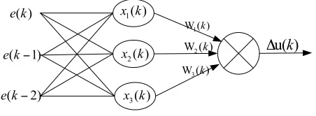
The structure of NNC. The NNC (neural network controller) is represented by the following structure, which is the three-layer neural network. The first layer of NNC is input layer, the input dataX(k)=[e(k),e(k!1),e(k!2)], where
e
(
k
)
represents thetracking error between real output and expected output at sample time
k
.)
(
)
(
)
(
k
y
*k
y
k
e
=
!
(12)where
y
*(
k
)
,y
(
k
)
represent the desired output and real output respectively.1( ) x k
3( ) x k
2( )
x k
!
u( )
k
1 W ( )k
2 W ( )k
3 W ( )k ( )
e k
( 1) e k"
( 2) e k"
Fig. 2. The inner structure of NNC
The second layer is the hidden layer which contains three neural units; the response of a neural unit is as follows.
!
"
!
#
$
%
+
%
%
=
&
=
%
%
=
&
=
=
)
2
(
)
1
(
2
)
(
)
(
)
(
)
1
(
)
(
)
(
)
(
)
(
)
(
2 3 2 1k
e
k
e
k
e
k
e
k
x
k
e
k
e
k
e
k
x
k
e
k
x
(13)The output of neural network controller
)
(
)
(
)
(
)
(
k
w
1x
1k
w
2x
2k
w
3x
3k
u
=
+
+
where
{ }
w
i,
i
=
,1
2
,
3
means the weight of neural network, when the appropriatevalue of the
w
i is selected, the controller usually can have a good performance.)
(
k
u
!
is variable rate of control law.u
(
k
)
=
u
(
k
"
1
)
+
!
u
(
k
)
is the control law at the sampling timek
. So the NNC has the structure of neural network PID control-ler.The weight of the neural network controller
{ }
w
i,
i
=
,1
2
,
3
can be trained by theoptimal objective function
[
*(
)
~
(
)
]
22
1
y
k
y
k
J
c=
!
. So[
(
)
~
(
)
]
(ˆ
)
(
)
)
(
-)
(
y
*k
y
k
k
x
k
w
k
J
k
w
ii c
i
"
=
"
#
!
$
$
=
%
(15)where
!
>
0
means the learning rate of neural network controller, andi
=
1
,
2
,
3
.)
(
)
1
-(
)
(
k
w
k
w
k
w
i=
i+
!
i means the weight of neural network controller at thesampling time
k
.3
The stability and convergence of control algorithm
In order to obtain the convergence and stability of the controller of nonlinear sys-tem, another assumption about the controlled system should be made.
A4: The PPD satisfies
"
c(
k
)
>
!
>
0
or"
c(
k
)
<
-
!
, and!
is a small positiveconstant. Without the loss of generality, it is assumed in this paper.
Theorem 1: The nonlinear system (1) satisfies Assumption 1-3, the estimation al-gorithm of model adopts the formula (5-6). The control rate adopts formula (15). If the expected output of nonlinear system is bounded, and the estimation of model is stable, and the control algorithm is stable. And the real output and input is bounded.
Proof
1) Time-varying parameter
!
ˆ( )
k
is bounded.Considering the length of article, the paper don’t give the detailed proof, the de-tailed process is stated in the paper[10].
2) The convergence of the nonlinear system model Define Lyapunov function
2 2
)]
(
[
)
(
k
=
s
k
+
!
V
(16)where
!
is a small positive const to guaranteeV
(
k
)
which is a positive function. According to the reaching-law of continuous sliding mode control, the reaching law of discrete-time sliding mode control can be written as[12].0
)
(
)
1
(
)
(
=
+
!
<
)
(
)
1
(
2
)
2
(
))
(
(
))]
(
sgn(
)
(
)
1
[(
))
(
(
-))
1
(
(
)
(
)
1
(
)
(
2 2 2 2k
s
qT
T
qT
qT
k
s
k
s
T
k
s
qT
k
s
k
s
k
V
k
V
k
V
!
!
!
!
=
!
!
!
=
+
=
!
+
=
"
#
#
(18)Since
1
>
qT
>
0
,!
,
q
,
T
>
0
, hence"
V
!
0
.According to the Lyapunov stability theorem, the identification model is stable. On the promise of the given initial value,
V
(
0
)
is bounded, using the control law (14), the estimation of model errore
(
k
)
tends to zero, this is0
)
(
)
(
)
(
~
)
(
lim
!
=
!
=
"
#
y
k
y
k
y
k
y
k
k .
3) The convergence of control algorithm
According to the approach ability of neural network, the network can optimize the parameters of controller by the error back-propagation way, so the output of controller can approach the desired output[13]. Define global Lyapunov function
2
))
(
(
*
5
.
0
)
(
k
e
k
V
g=
(19)2 2 2
))
(
(
*
5
.
0
)
(
*
)
(
))
(
(
*
5
.
0
))
(
)
(
(
*
5
.
0
)
(
k
e
k
e
k
e
k
e
k
e
k
e
k
V
g!
+
!
=
"
!
+
=
!
(20)As we all know,
e
(
k
)
is the function about the{
w
i}
, it also)
,
,
(
)
(
k
f
w
1w
2w
3e
!
. According to the principle of calculus, we can get the fol-lowing expression.[
]
!
!
!
!
!
= = ="
"
=
#
$
%
#
%
"
=
#
$
%
#
$
+
"
%
"
=
#
%
"
%
=
#
%
%
=
#
3 1 2 * 2 3 1 3 1 3 1 * 3 1))
(
(
*
)
(
~
)
(
))
(
ˆ
(
))
(
(
)
(
ˆ
))
(
)
(
ˆ
)
1
(
(
*
))
(
~
)
(
(
*
)
(
)
(
i ii i i
i i i
i i i i
k
x
k
y
k
y
k
w
w
k
u
k
w
w
k
u
k
k
y
w
w
k
y
k
y
w
w
k
e
k
e
&
'
&
&
(21)[
]
!
="
"
#
$
3 1 2 *2
(
)
(
)
*
(
(
))
))
(
ˆ
(
)
(
i ik
x
k
y
k
y
k
k
e
&
%
(22)According to the formula (20) and (22),
[
]
!
!
= ="
"
"
=
#
+
#
=
#
3 1 3 1 2 2 2 2 *2
(
)
(
)
(
(
))
[
1
0
.
5
*
(
(ˆ
))
*
(
(
))
]
))
(ˆ
(
))
(
*
5
.
0
)
(
)(
(
)
(
i i i i
g
k
x
k
k
x
k
y
k
y
k
k
e
k
e
k
e
k
V
$
%
$
%
(23) If!
="
3 1 2 2*
(
(
))
1
))
(
ˆ
(
2
1
i ik
x
k
#
$
, hence"
V
g(
k
)
!
0
, according to the principleof Lyapunov stability, the control system is stable.
Overall, the maximal tracking error of nonlinear system can be expressed
!
<
"
=
max
(
)
(
)
))
(
(
e
k
y
*k
y
k
Max
. In the range of allowable error, the controlsystem has a global convergence.
4) The boundness of real output and input
!
<
"
=
max
(
)
(
)
))
(
(
e
k
y
*k
y
k
Max
,e
(
k
)
is bounded, and the desired output isbounded. So the real output is bounded. Since the time-varying parameter
!
ˆ
(
k
)
is bounded, andu
(
k
)
"
!
1Max
(
y
(
k
)
)
+
!
2, and!
1,
!
2is a const. Henceu
(
k
)
is also bounded.Clearly, the Theorem 1 can be proved.
4
Simulation results
In this section, the two simulations are used to show the effectiveness and robust-ness of the control algorithm.
1.The convergence and superiority of algorithm compared with the traditional PID algorithm in linear system.
2.The convergence and robustness of control system in nonlinear system.
4.1 The convergence and robustness of algorithm in linear system
The convergence of algorithm in linear system. As we all known, the traditional PID algorithm is the most important control algorithm in linear system. The output of the incremental PID algorithm is
2
( )
p( )
i( )
d( ( ))
u k
k e k k e k k
e k
In order to verify the superiority compared with the traditional PID algorithm, the discrete-time linear system is defined as follows
( ) 0.8* ( 1) 0.5 (
2) 0.5 ( 1)
y k
=
y k
! !
y k
!
+
u k
!
(25)where
k
is a positive integer, and the desired output be written as (26)*( ) 1
40
y k
=
k
<
(26)Fig. 3. The tracking performance compared with traditional PID in linear system
The simulation diagram is showed in figure 3, as we can see, if the sampling time is less than 3, the controller needs to collect the error information of the tracking sys-tem, so the real output equal to zero; After three sample time, the control system can be stable in the finite time; the real output can track the desired output perfectly and the error of tracking can be in allowable range. The simulation results show the new algorithm can depress the overshoot compared with the traditional PID algorithm, decrease the adjustment time and get the satisfactory tracking performance.
The robustness of algorithm in linear system. The robustness of system is the important index in control systems, it refers to the perturbation of system parameters or system structure, the system still can maintain the characteristics, like convergence or stability. In order to verify the robustness of linear system compared with the tradi-tional PID algorithm, the simulation model is as follows, the parameters perturbation happens at sample time
k
=
30
.0.8* ( 1) 0.5 ( 2) 0.5 ( 1) 0.8* ( 1) 0.8 ( 2) 0.5 ( 1)
30 ( )
30
y k y k u k
y k y k u k
k y k
k
! ! ! + !
! ! ! + !
< "
= # >=
$
(27)
0 5 10 15 20 25 30 35 40
0 0.5 1 1.5
Sample time k
The s
ys
tem
out
put
Fig. 4. The robustness of algorithm compared with traditional PID algorithm in linear system
As we can see in the figure 4, when the structure parameters of system change at the sample time
k
=
30
, the new algorithm still has the better tracking performance, and the tracking error can be in the range of allowable at the finite time. And the ad-justment time and adad-justment amplitude of new algorithm can be smaller during the period of the system parameters perturbation compared with traditional PID algo-rithm.4.2 The convergence and robustness of nonlinear system
The convergence and superiority compared with the MFAC algorithm. MFAC (model free adaptive control), as we know, has the good performance in the nonlinear control system. So, in order to verify the superiority, we compare with the MFAC algorithm. The discrete-time nonlinear system
3
2
(
(
))
))
1
(
(
1
)
1
(
)
(
u
k
k
y
k
y
k
y
+
!
+
!
=
(28)where u(k) is the control variable of controller, y(k)and y(k!1) are the current and
the one step delayed outputs, respectively. And the desired output of the system is as follows:
*
0.5sin( 500) 0.3cos( 500)... 1000 ( ) 0.3...1500 1000
0.3... 1500
k k k
y k k
k ! + ! <
" #
=$ > >=
#% >=
&
(29)
0 10 20 30 40 50 60
0 0.5 1 1.5
Sample time k
The s
ys
tem
out
put
(a) the comparative figure between new algorithm and MFAC algorithm
(b) Local enlarged figure of simulation results
Fig. 5. The superiority of control system compared with the MFAC algorithm
As we can see from the figure 5(a), the tracking error of system can be ignored in the range of error allowed except the sudden change of desired output. The simulation result validates the convergence of the algorithm and the stability of the system identi-fication in nonlinear system. As shown in the local enlarged figure 5(b), the MFAC and new algorithm can track the desired output after the several step times. And the adjustment time and adjustment amplitude of the new algorithm have a great im-provement compared with the MFAC algorithm.
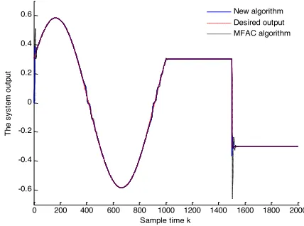
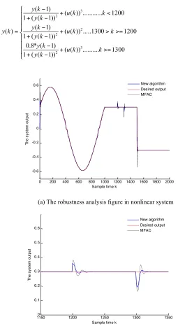
The robustness of control system. In order to verify the robustness of the algo-rithm, the paper adopts the same control parameters to validate the robustness of the
0 200 400 600 800 1000 1200 1400 1600 1800 2000 -0.6
-0.4 -0.2 0 0.2 0.4 0.6
Sample time k
The s
ys
tem
out
put
New algorithm Desired output MFAC algorithm
0 20 40 60 80 100 120 140 160 180 200 -0.6
-0.4 -0.2 0 0.2 0.4 0.6
Sample time k
The s
ys
tem
out
put
new control algorithm; the tracking performance is shown in the figure 6. The simula-tion model is adopted (30), and the desired output is as the form of (29).
3 2
2 2
3 2
( 1) ( ( )) ... 1200 1 ( ( 1))
( 1)
( ) ( ( )) ...1300 1200
1 ( ( 1))
0.8* ( 1) ( ( )) ... 1300 1 ( ( 1))
y k u k k
y k y k
y k u k k
y k
y k u k k
y k ! "
+ <
# + " #
# "
=$ + > >=
+ " #
# "
+ >=
#
+ "
% (30)
(a) The robustness analysis figure in nonlinear system
(b) The local enlarged figure between new algorithm and MFAC algorithm
Fig. 6. The robust analysis in the nonlinear system
0 200 400 600 800 1000 1200 1400 1600 1800 2000 -0.6
-0.4 -0.2 0 0.2 0.4 0.6
Sample time k
The s
ys
tem
out
put
New algorithm Desired output MFAC
11500 1200 1250 1300 1350
0.1 0.2 0.3 0.4 0.5 0.6
Sample time k
The s
ys
tem
out
put
As we can see in the figure 6, when the structure parameters of system change at the sampling time k=1200,
k
=
1300
, the algorithm still has the better tracking performance, and the tracking error can be in the range of allowable at the finite time. From the local enlarged figure 6(b), we can see that the adjustment time and adjust-ment amplitude of the new algorithm is less than the MFAC algorithm.5
Conclusion
In this paper, a new dynamic linearization model about the Quasi-Sliding Mode al-gorithm was proposed for identification of complex nonlinear system. A neural net-work PID controller is designed to get the optimized control rate based on the above model. The advantages of algorithm are as follows:
1.better robustness
2.better tracking performance 3.less adjustment time and amplitude.
And the global stability of the system is proved by the way of the Lyponou func-tion and Matlab simulafunc-tion.
6
Acknowledgment
The work is supported by the National Science and technology support program (NO 2014BAG06B02) and Fundamental Research Funds for the Central Universities (No 2014HGCH0003).
7
References
[1]Ding, Feng. "Hierarchical multi-innovation stochastic gradient algorithm for Hammerstein nonlinear system modeling." Applied Mathematical Modelling 37.4 (2013): 1694-1704.
https://doi.org/10.1016/j.apm.2012.04.039
[2]Nigam, Vivek Prakash, and Daniel Graupe. "A neural-network-based detection of epilep-sy." Neurological Research 26.1 (2004): 55-60. https://doi.org/10.1179/01616410 4773026534
[3]Wang, Tong, Huijun Gao, and Jianbin Qiu. "A combined adaptive neural network and non-linear model predictive control for multirate networked industrial process control." IEEE Transactions on Neural Networks and Learning Systems 27.2 (2016): 416-425.
https://doi.org/10.1109/TNNLS.2015.2411671
[4]Li, Hongyi, et al. "Control of nonlinear networked systems with packet dropouts: interval type-2 fuzzy model-based approach." IEEE Transactions on Cybernetics 45.11 (2015): 2378-2389. https://doi.org/10.1109/TCYB.2014.2371814
[6]Hou, Yi-You, and Zhang-Lin Wan. "Robust Stability for Nonlinear Systems with Time-Varying Delay and Uncertainties via the Quasi-Sliding Mode Control." International Jour-nal of Antennas and Propagation 2014 (2014). https://doi.org/10.1155/2014/897179
[7]Ma, Haifeng, Jianhua Wu, and Zhenhua Xiong. "Discrete-time sliding-mode control with improved quasi-sliding-mode domain." IEEE Transactions on Industrial Electronics 63.10 (2016): 6292-6304. https://doi.org/10.1109/TIE.2016.2580531
[8]Zhu, Yuanming, and Zhongsheng Hou. "Data-driven MFAC for a class of discrete-time nonlinear systems with RBFNN." IEEE transactions on neural networks and learning sys-tems 25.5 (2014): 1013-1020. https://doi.org/10.1109/TNNLS.2013.2291792
[9]Ma, Ping, et al. "Main steam temperature control system based on MFAC." Electric Power Science and Engineering 1 (2006): 006.
[10]Cheng, Zhihui, Zhongsheng Hou, and Shangtai Jin. "MFAC-based balance control for freeway and auxiliary road system with multi-intersections." Control Conference (ASCC), 2015 10th Asian. IEEE, 2015.
[11]Han, Yueqiao, Yonggui Kao, and Cunchen Gao. "Robust sliding mode control for uncer-tain discrete singular systems with time-varying delays and external disturbances." Auto-matica 75 (2017): 210-216. https://doi.org/10.1016/j.automatica.2016.10.001
[12]Sarpturk, S. Z., Yorgo Istefanopulos, and Okyay Kaynak. "On the stability of discrete-time sliding mode control systems." IEEE Transactions on Automatic Control 32.10 (1987): 930-932. https://doi.org/10.1109/TAC.1987.1104468
[13]Mukhopadhyay, Snehasis, and Kumpati S. Narendra. "Disturbance rejection in nonlinear systems using neural networks." IEEE Transactions on Neural Networks 4.1 (1993): 63-72. https://doi.org/10.1109/72.182696
[14]Chandrasena Premawardhena, N., ICT in the foreign language classroom in Sri Lanka: A journey through a decade. 10th World Conference on Computers in Education (WCCE 2013), Nicolaus Copernicus University, July 2-5 2013, Torun, Poland.pp 223-224
8
Authors
Huifang Kong is the Professor and the Director of the Research Center of Auto-motive Electronics and Control Technology in Hefei University of Technology, No 193, Tunxi Road, Hefei, China, 230009. Her research interests including Control Engineering, Industrial Automation, and Dynamics and Control. ([email protected]).
Yao Fang is a PH.D student in the Automotive Electronics and Control Research Center in Hefei University of Technology, Majoring in modeling and control of com-plex nonlinear systems!Energy management of hybrid electric vehicle and the
behav-ior decision of drivers.