KANTOROVICH-EULER LAGRANGE-GALERKIN’S METHOD FOR
BENDING ANALYSIS OF THIN PLATES
C. C. Ike*
DEPT. OF CIVIL ENGINEERING, ENUGU STATE UNIVERSITY OF SCIENCE & TECHNOLOGY, ENUGU. ENUGU STATE. NIGERIA
E-mail address:
[email protected]
ABSTRACT
In this work, the Kantorovich method is applied to solve the bending problem of thin rectangular plates with three simply supported edges and one fixed edge subject to uniformly distributed load over the entire plate surface. In the method, the plate bending problem is presented using variational calculus. The total potential energy functional is found in terms of a displacement function constructed using the Kantorovich procedure, as the product of an unknown function of x (f(x)) and a coordinate basis function in the y direction that satisfies the displacement end conditions at y = 0, y = b. The Euler-Lagrange differential equation is determined for this functional. The Galerkin method is then used to obtain the unknown function f(x). Bending moment curvature relations are used to find the bending moments and their extreme values. The results obtained agree remarkably well with literature. The effectiveness of the method is demonstrated by the marginal relative error obtained for one term displacement solutions.
Keywords: Kantorovich-Galerkin, thin plate, potential energy functional, Euler-Lagrange differential equation.
1. INTRODUCTION
Plates are initially flat structural members bounded by two parallel planes, called faces and rectilinear or curvilinear surface called an edge or boundary. The generators of the cylindrical surface are perpendicular to the plane faces. The distance between these plane faces is called the thickness h, which is small as compared with the other characteristic dimensions of the plate [1]. Geometrically, plates are bounded by either rectilinear or curved boundaries. Plates are widely used in the fields of aerospace, aeronautical, naval, marine, mechanical, architectural, structural, and highway engineering. Specifically, plates are used in architectural structures, bridge decks, naval and marine structures, containers, airplane panels, spacecraft panels, missiles, ship decks, instruments, machine parts (components) and hydraulic structures. They are classified by their shapes as rectangular, circular, elliptical, square, triangular, sector, circular with hole, square with hole, etc. They are also classified according to their materials of construction as homogeneous, heterogeneous, isotropic, anisotropic, and orthotropic.
The structural behavior of plates as a function of the type of loading acting on it can be classified as static flexure, dynamic flexure or buckling. The analysis of the plates for static flexure, dynamic flexure, and buckling has been extensively done in the technical literature [2 – 9].
The analysis of plates has generated considerable research interest and activities, with many varying methods being developed and implemented for specific shape and material properties. The methods for plates analysis can be grouped into two namely: analytical methods and numerical or approximate methods. Analytical methods of plate analysis seek to find mathematical expressions valid for the entire plate region that identically solve the governing partial differential equations on the entire plate domain subject to the geometric and natural boundary conditions at the plate edges. They are closed form mathematical solutions which exist for a limited number of plate problems, and for the vast majority of plate problems whether in static flexure, dynamic flexure or buckling, they do not exist [10 - 13]. The need for approximate solutions for cases where closed form analytical solutions cannot be found gave rise to numerical methods for solving plate problems. The double trigonometric or Fourier series method was one of the earliest methods of solving the plate problem. The method, applicable to plates with all edges simply supported, assumes, apriori, that a double Fourier series can be developed to represent any distribution of the applied load p (x, y). By assuming that the deflection response can be represented by a double Fourier series of the same form as the loading, and which is specifically constructed to satisfy the geometric and force boundary conditions at the simply supported
Vol. 36, No. 2, April 2017, pp. 351 – 360
Copyright© Faculty of Engineering, University of Nigeria, Nsukka,
Print ISSN: 0331-8443, Electronic ISSN: 2467-8821
www.nijotech.com
edges, the governing fourth order biharmonic equation for flexural static analysis of thin plates is simplified to an algebraic problem, readily solved to find the unknown generalized displacement parameters. Thus, the internal forces are obtained from the internal force displacement relations.
Levy’s single trigonometric series method was originally developed for the analysis of rectangular thin plates with two opposite edges simply supported; and the remaining two edges subject to arbitrary boundary support conditions. Levy chose the x and y coordinate axes such that the plate surface is defined by ⁄ ⁄ where the edges x = 0, x = a are simply supported [15]. He then assumed the deflection can be represented as a single Fourier series that automatically satisfies the simply supported boundary conditions along the edges x = 0, x = a; regardless of the choice of fm(y)
which must be obtained such as to satisfy homogeneous part of the plate equation and also satisfy the support conditions at ⁄ He further assumed, in line with the theory for non-homogeneous differential equations, that the general solution of the governing equation is the superposition of the homogeneous solution wh and the
particular solution wp.
The primary attraction of Levy’s method is the advantage presented by a single Fourier series representation of the plate deflection and load distribution, which is convenient and efficient from the perspective of mathematical analysis, and computations [10].
The method is particularly suited to the rectangular thin plate problems with simple support on two opposite edges and arbitrary support conditions in the remaining two edges [16]. It is more general in application than the double trigonometric series method, and the resulting series for deflection converges more rapidly. However, the computational rigours and demands are more in the single trigonometric series method than the double trigonometric series method.
Apart from the analytical methods of Navier and Levy, many numerical and approximate methods have been formulated and implemented for the analysis of plates under static flexure, dynamic flexure and buckling. Such methods include variational methods (Ritz, Galerkin, Kantorovich), Weighted residual methods (Point collocation, Galerkin method, Bubnov-Galerkin method, subdomain collocation, Least squares residual). Virtual work methods, Finite Difference method, Improved Finite Difference method, Boundary Element method, Finite Element method, Symplectic Elasticity method and Finite Strip method. Researchers have used various numerical methods to solve plate problems [ 3 – 8, 17 – 1 9, 21].
The general aim of this research is to apply the Kantorovich-Galerkin method to the static flexural analysis of rectangular Kirchhoff plates with three simply supported edges and one clamped edge, for the case of uniformly distributed load over the entire plate surface. The specific objectives are:
(i) to present the methodology of the Kantorovich-Galerkin method for the rectangular thin plate problem
(ii) to determine the Euler-Lagrange differential equation of equilibrium for the Kirchhoff plate with three simply supported edges and one clamped edge for the case of uniformly distributed load over the entire plate surface
(iii) to formulate the Galerkin variational integral equation for the Euler-Lagrange differential equation of equilibrium
(iv) to solve the Galerkin variational integral statement, and obtain the unknown function f(x) in the assumed displacement function
(v) to find the critical values of the displacement, and use the bending moment curvature equations to find the bending moment distributions, and critical values of the bending moment.
2. APPLICATION OF KANTOROVICH-EULER-GALERKIN METHOD TO THE BENDING ANALYSIS OF CSSS PLATE Consider a rectangular Kirchhoff plate that is simply supported at the edges x = 0, x = a, y = b, and clamped at the edge y = 0. The plate is subject to a uniformly distributed transverse load of intensity p over the entire plate domain , , as shown in Figure. 1.
Fig.1: Rectangular Kirchhoff CSSS plate under uniformly distributed load
A suitable displacement function that satisfies the boundary conditions at the edges y = 0, y = b is obtained by considering the fourth degree polynomial function
( ) ( ) In (1), are unknown polynomial constants, and b is the span of the plate in the y
determined such that g(y) should become a suitable polynomial shape function for the plate in the y
coordinate direction. Hence g(y) is required to satisfy the boundary conditions:
( ) ( )
( ) ( ) ( )
where ( )
( )
( )
( ) ( )
( ) ( )
Using the boundary conditions,
( )
( )
( )
th s ( ) ( )
( ) ( )
or ( ) ( ) ( )
By the Kantorovich-Galerkin method, we assume for the plate flexure problem
( ) ( ) ( ) ( )
and then determine f(x) for w(x, y) to be a true displacement function of the plate.
. __________________________________________________________________ The total energy functional is given by:
∬ [( ) ( )( )] ∬ ( )
where R is the two dimensional plate domain.,
is the Poisson’s ratio andBy Kantorovich-Galerkin method, the total energy functional should be minimized for equilibrium of the plate under static flexure. Due to the support conditions of the plate the twisting curvatures vanish and the total energy functional simplifies to Equation (13) as follows:
∬ ( ) ∬ ( )
Using the assumed displacement function, the total energy functional becomes
∫ ∫ {[ ( ) ( )]} ∫ ∫ ( ) ( ) ( )
Simplifying, we obtain:
∫ ∫ {( ) ( ( )) ( )( )
( ) ( )
( )
( ( )) } ∫ ∫ ( ) ( ) ( )
Further simplification and evaluation of integrals yields the total energy functional to be minimized as Equation(16)
∫ [ ( ( )) ( )
( )
( ( )) ( )] ( )
The integrand in the total energy functional is ( ( ) ( )) where
( ( ) ( )) ( ( )) ( )
( ) ( ( ))
( ) ( )
2.1 Euler-Lagrange Differential Equation for the Functional
The Euler-Lagrange differential equation for this functional is: [22, 23, 24]
(
( )) (
( )) ( )
Applying the Euler-Lagrange condition, we find the condition for the extremum of the total energy functional as the fourth order ordinary differential equation in f(x) as follows:
Simplifying, Equation (19) can be written as:
( ) ( ) ( ) ( )
2.2 Galerkin Solution to the Euler-Lagrange Equation
The ordinary differential equation, Equation (12), is solved subject to the boundary conditions at the simply supported ends x = 0, x = a. A suitable displacement shape function f(x) that satisfies the boundary conditions of simple supports at the edge x = 0, x = a, i.e. f(0) = 0, f(a) = 0, ( ) = 0, f ” (a) = 0 is obtained by considering the fourth degree polynomial f4(x) as follows:
( ) ( ) where c0, c1, c2,c3 and c4 are the polynomial constants obtained by requiring that f(x) satisfies the boundary conditions
at x = 0, x = a. Thus, using the boundary conditions,
( ) ( )
and ( ) ( ) ( )
The other higher shape functions are obtained from f(x) by multiplication by x, x2, x3 … xn.
However xf(x) satisfies the displacement boundary condition at x = 0, x = a, but violates the force boundary condition atx = 0, x = a. (M(x = 0) = M(x = a) = 0) where Mx is the bending moment. Thus, in general,
( ) ( ) ( ) ( )
where c1, c2, c3 … cn are the n undetermined parameters of f(x). For a one parameter solution for f(x),f(x) is considered
as:
( ) ( ) ( )
A Galerkin variational solution is sought to the Euler-Lagrange differential equation in order to obtain the parameter c1.
The Galerkin variational integral becomes:
∫ ( ( ) ( ) ( ) ) ( ) ( )
∫ ( ( ) ( ) ) ( ) ( )
Simplifying, we obtain
{ ∫ ( ) ∫ ( ) ( )
∫ ( ) } ∫ ( ) ( )
( )
Let ⁄
(
)
( )
( ) ( ) where ( ) ( ) ( )
Thus, the deflection function along x-axis becomes:
( ) ( ) ( ) ( ) ( )
( ) ( ) ( ) ( ) ( ) ( )
( ) ( ) ( ) ( )
2.3 Two-Term Displacement Shape Function in Polynomial form in the Kantorovich Functional
Substituting the second term deflection function into the Euler-Lagrange differential Equation; and evaluating for the constants, c1 and c2 sing the Galerkin’s variational integral gives:
∫ [ ( ) ( ) ( ) ] ( ) ( )
where i = 1, 2, and;
( ) ( ) ( ) ( )
where ( ) ( ) ( ) Thus, Equation (37) becomes:
{ ∫ ∫ ∫ } { ∫ ∫
∫ } ∫ ( )
{ ∫ ∫ ∫ }
{ ∫ ∫ ∫ } ∫ ( )
Evaluating the integrals, we obtain:
( ) ( ) ( )
( ) ( ) ( )
( ) ( ) ( )
( ) ( ) ( )
________________________________________________ In compact form, Equation (45) becomes:
( ) ( )
where,
( )
( )
( )
( ) ( ) ( )
By Cramer’s r le
( )
|
| ( )
|
| ( )
|
| ( )
Th s f( ) c c
2.4 Center Deflection
The deflection at the center of the plate is found as:
( ⁄ ⁄ ) ( )| ( )| ( )
( )
( )
where
2.5 Bending Moments
The bending moment distributions are given by Timoshenko and Woinowsky-Krieger [12] as;
( ) ( ) ( )
where
( ) ( )
At the center of the plate,
(
) ( )
(
) ( )
( )
(
) ( )
( )( ) ( ) ( )
Similarly,
( ) ( )
( )
(
) ( )
( ) (
) ( )
( ) (
) ( )
( ) (
) ( )
2.6 Alternative Expressions for Bending Moments
The bending moments expressions for rectangular plates under pure bending along x and y axes are given by Timoshenko and Woinowsky-Krieger [12] as Equation (59).Substituting Equation (36) into Equation (59), we obtained the first term approximation to the bending moment expressions for rectangular plates under bending along x and y axes as follows:
______________________
( ) ( ( ) ( ) ( ) ( )) ( )
( ) ( ( ) ( ) ( ) ( )) ( )
At mid-span of the plate; Equations (34 and 35) become:
( ) ( (
) (
) (
) (
)) ( )
( ) ( (
) ( ) ( ) ( )) ( )
( ) ( ( )
( )) ( )
( ) ( )
where,
b
a
;
( ) (
( ) ) ( )
( ) ( ) ( )
Similarly,
( ) ( ) ( )
where,
( ) ( ) ( ) ( ) ( ) The solutions for deflection coefficients and bending moment coefficient are presented in Tables 1, 2, 3, 4, and 5. At the center of the plate, the deflection can be obtained as
( ) | ⁄ ( ⁄ ) ( )
(
) ( ) The bending moment distributions are found from Equation (59).
At the center of the plate,
(
) (
) ( )
[( ) ( ) ( ) ( ) ] ( ) ( ( ( ) ( )) ( ( ) ( )) ( )
At the plate center, ⁄ ⁄
(
( ) ) (
( ) (
) ) ( )
(
) (
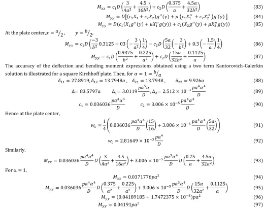
) ( ) The accuracy of the deflection and bending moment expressions obtained using a two term Kantorovich-Galerkin solution is illustrated for a square Kirchhoff plate. Then, for ⁄
( )
( )
( )
Hence at the plate center,
( (
)
(
)) ( )
( )
Similarly,
(
)
(
) ( ) For = 1,
( )
( ) (
) ( )
( ) ( ) ( )
3. RESULTS AND DISCUSSIONS
The Kantorovich-Galerkin variational method has been successfully implemented in this work to analyse the static flexure problem of a thin rectangular plate with three simply supported edges and one fixed (clamped) edge; and subject to uniformly distributed load over the entire plate surface. The displacement function was assumed following Kantorovich method to be a product of an unknown function of one spatial coordinate, x, and a coordinate basis function f(y) presented in Equation (11) which satisfies the boundary conditions at the edges
y = 0, y = b. The total potential energy functional was then found as given in Equation (16) to be a function of x, ( ) ( ) Using the principles of variational calculus,
the Euler-Lagrange differential equation of equilibrium was found for the extremization of the functional as the fourth order ordinary differential equation presented as Equation (19).
A Galerkin variational (weighted residual) solution to the Euler-Lagrange differential equation of equilibrium was then obtained for a one parameter choice of f(x). Thus the solution for w(x, y) to the plate flexure problem was
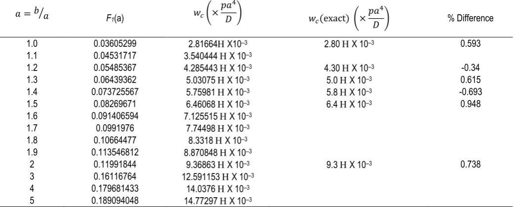
obtained as Equation (36). Bending moment expressions were then determined for the plate as Equations (64) and (70). Tables 1, 2, and 3 present the Kantorovich-Galerkin solutions for a one parameter assumption for the deflection and bending moment values of the centre of the plate and their comparison with exact solutions obtained by Timoshenko and Woinowsky-Krieger [12]. Table 1 shows that the relative difference between the Kantororich-Galerkin solutions and the exact solutions for displacement vary from 0.34% to 0.948% with an average value of 0.4%. The relative difference for bending moment coefficients βxx βyy as shown in Tables
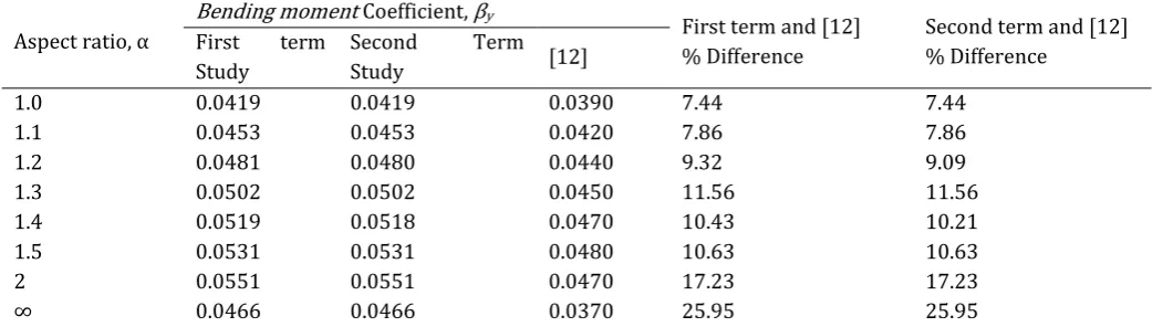
2 and 3 for a one parameter Kantorovich-Galerkin solution vary from 4.6% to 9.41%, for βxx and 7.46% to
17.23%, for βyy for the aspect ratio varying from 1.0 to
2.0.
becomes identical with the results obtained for the one term solutions. Two term (parameter) solutions yielded bending moment values given by Equation (94) for Mxx
and Equation (97) for Myy. Bending moment values given
by the two term solution yielded identical results with the one term solutions. The accuracy and effectiveness of the Kantorovich-Galerkin method is thus validated. The results of the study for deflections and bending moment at the mid – span of the CSSS plate is tabulated in Tables 1, 2, 3, 4, 5 and 6 for first and second terms approximation to the deflection functions respectively. These values which are computed at aspect ratio range: α and Poisson ratio µ (steel material)
represent deflection function coefficients, and bending moment coefficients about x and y directions, and respectively. Results from Timoshenko and Woinowsky – Krieger [12] were also tabulated alongside these values; and percentage differences between them were calculated as:
percentage difference
( al e o tained y a theory corresponding val e y e act theroy) ( )
The results are presented in Tables 1, 2, and 3.
Table 1: Deflection coefficients for deflection at the center of CSSS plates under uniform load (one term Kantorovich-Galerkin solution)
⁄ F
1(a) (
)
(e act) ( ) % Difference
1.0 0.03605299 2.81664Х10–3 2.80 Х 10–3 0.593
1.1 0.04531717 3.540444 Х 10–3
1.2 0.05485367 4.285443 Х 10–3 4.30 Х 10–3 -0.34
1.3 0.06439362 5.03075 Х 10–3 5.0 Х 10–3 0.615
1.4 0.073725567 5.75981 Х 10–3 5.8 Х 10–3 -0.693
1.5 0.08269671 6.46068 Х 10–3 6.4 Х 10–3 0.948
1.6 0.091406594 7.125515 Х 10–3
1.7 0.0991976 7.74498 Х 10–3
1.8 0.10664477 8.3318 Х 10–3
1.9 0.113546812 8.870848 Х 10–3
2 0.11991844 9.36863 Х 10–3 9.3 Х 10–3 0.738
3 0.16116764 12.591153 Х 10–3
4 0.179681433 14.0376 Х 10–3
5 0.189094048 14.77297 Х 10–3
Table 2: Bending moment coefficient βxx for the center of
CSSS plate under uniformly distributed load (one-term Kantorovich-Galerkin solution)
⁄ ( ) (e act)( ) % Difference
1.0 0.0371797 0.034 9.41 1.1 0.04452 0.041 8.59 1.2 0.051854 0.049 5.82 1.3 0.0590 0.056 5.36 1.4 0.06587 0.063 4.56 1.5 0.07236 0.069 4.87 1.6 0.07843
1.7 0.08405 1.8 0.08924 1.9 0.094
2 0.098372 0.094 4.68
Table 3: Bending moment coefficient βyy for the center of
CSSS plate under uniformly distributed load (one-term Kantorovich-Galerkin solution)
⁄ ( ) (e act)( ) Difference %
1.0 0.04191 0.039 7.46 1.1 0.0453 0.042 7.86 1.2 0.04805 0.044 9.20 1.3 0.05021 0.045 11.58 1.4 0.05185 0.047 10.32 1.5 0.05306 0.048 10.54 1.6 0.05392
1.7 0.0545 1.8 0.05485 1.9 0.0550
Table 4: Mid – span deflection coefficients (for four decimal places)
Aspect ratio α
Deflection Coefficient λ
First term and [12] % Difference
Second term and [12] % Difference
First term Study
Second Term Study [12]
1.0 0.0028 0.0028 0.0028 0.00 0.00 1.1 0.0035 0.0035 0.0035 0.00 0.00 1.2 0.0043 0.0043 0.0043 0.00 0.00 1.3 0.0050 0.0050 0.0050 0.00 0.00 1.4 0.0058 0.0058 0.0058 0.00 0.00 1.5 0.0065 0.0065 0.0064 1.56 1.56 2 0.0094 0.0094 0.0093 1.08 1.08 ∞ 0.0162 0.0162 0.0130 24.62 24.62
Table 5: Mid – span bending moment coefficients along x – a is βx (for four decimal places)
Aspect ratio α
Bending moment Coefficient, βx
First term and [12] % Difference
Second term and [12] % Difference
First term Study
Second Term Study [12]
1.0 0.0372 0.0372 0.0340 9.41 9.41 1.1 0.0445 0.0445 0.0410 8.54 8.54 1.2 0.0519 0.0518 0.0490 5.92 5.71 1.3 0.0590 0.0590 0.0560 5.36 5.36 1.4 0.0659 0.0659 0.0630 4.60 4.60 1.5 0.0724 0.0724 0.0690 4.93 4.93 2 0.0984 0.0984 0.0940 4.68 4.68 ∞ 0.1554 0.1554 0.1250 24.32 24.32
Table 6: Mid – span bending moment coefficients along y – a is βy (for four decimal places)
Aspect ratio α
Bending moment Coefficient, βy
First term and [12] % Difference
Second term and [12] % Difference
First term Study
Second Term Study [12]
1.0 0.0419 0.0419 0.0390 7.44 7.44 1.1 0.0453 0.0453 0.0420 7.86 7.86 1.2 0.0481 0.0480 0.0440 9.32 9.09 1.3 0.0502 0.0502 0.0450 11.56 11.56 1.4 0.0519 0.0518 0.0470 10.43 10.21 1.5 0.0531 0.0531 0.0480 10.63 10.63 2 0.0551 0.0551 0.0470 17.23 17.23 ∞ 0.0466 0.0466 0.0370 25.95 25.95
4. CONCLUSIONS
The analysis of CSSS plate has been investigated using Kantorovich – Euler Lagrange – Galerkin’s approaches for one and two unknown parameters approximation to deflection functions. The following inferences are therefore adduced:
a) Tr ncation of Taylor Macla rin’s infinite series beyond the fifth term (fourth degree) would result in higher terms of unknown parameters in the polynomial functions representation of the displacement coordinate functions.
b) Convergence of deflection and bending moments of CSSS plate to the exact solution did not improve with the use of the second parameter of the polynomial shape functions using the Kantorovich – Euler Lagrange method because the second shape function
violated force boundary conditions at the ends of the plate.
c) The use of one and two unknown parameters in the polynomial shape functions in the Kantorovich – Euler Lagrange – Galerkin method for CSSS plate gives marginally better solutions for deflections than for bending moments. However, the extent of difference for bending moments is approximately a single digit.
5. REFERENCES
[1] Kapadiya H. M. and Patel A. D. . Review of Bending Solutions of Thin Plates. International Journal of Scientific Research and Development (IJSRD) vol 3 Issue 03, 2015, ISSN:2321-0613, pp. 1709-1712. 2015.
[2] Sebastian V. K. An Elastic Solution for simply supported Rectangular Plates. Nigerian Journal of Technology Vol. 7 No.1 September, 1983, pp11-16. 1983.
[3] Osadebe N. N., Ike C. C., Onah H., Nwoji C. U. and Okafor F. O. Application of the Galerkin-Vlasov method to the Flexural Analysis of simply supported Rectangular Kirchhoff Plates under uniform loads. Nigerian Journal of Technology
Vol.35 October 2016.
[4] Ezeh J. C., Ibearugbulem O. M. and Onyechere C. I.. Pure Bending Analysis of Thin Rectangular Flat Plates using Ordinary Finite Difference Method. International Journal of Emerging Technology and Advanced Engineering, Volume 3, Issue 3, March, 2013 (www.ijetae.com ISSN: 2250-2459) 2013. [5] Aginam C. H., Chidolue C. A. and Ezeagu C. A.
Application of Direct Variational Method in the Analysis of Isotropic thin Rectangular Plates. ARPN Journal of Engineering and Applied Sciences, Vol.7, No.9, September, 2012. Asian Research Publishing Network (ARPN), 2012.
[6] Ibearugbulem O. M., Ettu, L. O., and Ezeh J. C. Direct Integration and Work Principle as New Approach in Bending Analysis of Isotropic Rectangular Plates.
The International Journal of Engineering and Science, Volume 2, Issue 3, pp. 28-36, 2013, ISSN 2319 -1813. 2013.
[7] Ibearugbulem O. M., Osadebe N. N., Eze J. C. and Onwuka D. O. Buckling Analysis of Axially Compressed SSSS thin Rectangular Plate using Taylor-Maclaurin shape function. International Journal of Civil and Structural Engineering, Volume 2, No.2, 2011, 2011.
[8] Umeh M. I. . Analysis of Isotropic and Orthotropic Plates by Polynomial Sphine Functions. PhD Thesis University of Nigeria, Nsukka, 1996.
[9] William T. S. Analysis of Plate on Elastic Foundations. PhD Thesis, Graduate Faculty of Texas Tech University, May 1990.
[10] Szilard R. Theories and Applications of Plate Analysis: Classical, Numerical and Engineering Methods. John Wiley and Sons Inc. 2004.
[11] Mansfield E. H. The Bending and Stretching of Plates, Macmillan, New York. 1964.
[12] Timoshenko S. P. and Woinowsky-Krieger S. Theory of Plates and Shells, 2nd Edition, McGraw Hill Book Co. New York. 1959.
[13] Ventsel E. and Krauthamner T. Thin Plates and Shells: Theory, Analysis and Applications, Marcel Dekker Inc. USA. 2004.
[14] Navier C. L. M. N. Bulletin des Science de la Societie philomartrique de Paris, 5, pp. 95-102. Extrait des recherché sur la flexion des planes elastiques. 1823. [15] Levy M. Memoire sur la theorie des plaques elastiques planes. Journal de mathematiques Pures et Appliquées; Vol 30 pp.219-306. 1899.
[16] Ugural A. C. Stresses in plates and shells, 2nd Edition, WCB McGraw Hill Boston. 1999.
[17] Balasubramanian Ashwin Plate Analysis with Different Geometries and Arbitrary Boundary Conditions. MSc. Thesis, Mechanical Engineering , Faculty of Graduate School, the University of Texas at Arlington, December, 2011.
[18] Sader J. E. and White L. Theoretical analysis of the static deflection of plates for atomic force microscope applications. J. Applied Physics, Vol. 14 No.1, 1 July 1993, pp.1-9.
[19] Gould P. L. Analysis of Shells and Plates. Springer-Verlog, New York Berlin. 1988.
[20] Reissner E. The Effect of Transverse Shear Deformation on the Bending of Elastic Plates.
Journal of Applied Mechanics, Vol 12, pp. A69. 1945. [21] Kantorovich L. V. and Krylov V. L. Approximate Methods of Higher Analysis. John Wiley and Sons, New York. 1954.
[22] Olver P. J. Introduction to the calculus of variations.
www.users.math.umu.edu./~olver/ln_/.cv.pdf 2016
[23] Mierseman E. Calculus of variations. Lecture notes, Department of Mathematics, Leipzig University, October 2012.
[24] Gelfard I. M. and Fomin S. V. Calculus of variations