Towards multi-purpose IS radar experiments

© European Geosciences Union 2008

Geophysicae

Towards multi-purpose IS radar experiments

I. I. Virtanen1, M. S. Lehtinen2, and J. Vierinen2

1_{Department of Physical Sciences, University of Oulu, P.O. Box 3000, 90014, Finland} 2_{Sodankyl¨a Geophysical Observatory, 99600, Sodankyl¨a, Finland}

Received: 20 December 2007 – Revised: 17 March 2008 – Accepted: 4 June 2008 – Published: 5 August 2008

Abstract. The EISCAT incoherent scatter radars routinely perform simultaneous measurements of E- and F-regions of the ionosphere. In addition several experiments exist for measuring pulse-to-pulse correlations from the D-region. However, the D-region experiments have quite limited range extents and the short lags suffer from F-region echoes, which are difficult to properly handle with standard decoding meth-ods.

In this paper it is demonstrated with real data how D-region experiments can be designed to produce continuous lag profiles extending above the F-region maximum. The large range coverage is attained for all lags shorter than the longest transmission pulse and it allows one to properly in-clude the F-region echoes in the analysis. The large cov-erage is not needed for pulse-to-pulse lags because E- and F-regions do not have this long correlation times. The lag profiles with large range extent also provide a useful mea-surement of the upper parts of the ionosphere.

The experiments utilise new kind of phase coding tech-nique, which has estimation accuracy comparable to that of alternating codes though the code sequence is very short. No special decoding method is applied to the codes, because the lag profile inversion method automatically adapts to any kind of transmission codes provided transmission samples are available.

The computing resources needed for real-time lag profile inversion with two different kinds of goals are also discussed here: 1) real-time monitoring of the results and 2) use of in-verted lag profiles as a way to permanently store the data. While it was possible to accomplish real-time monitoring with a standard high-end desktop workstation, the higher res-olution requirement for permanent data storage purposes is a much more critical task, requiring the use of larger-scale par-allel processing.

Keywords. Radio science (Ionospheric physics; Signal pro-cessing; Instruments and techniques)

Correspondence to: I. I. Virtanen ([email protected])

1 Introduction

A common way to arrange transmission pulses in incoherent scatter radar (ISR) experiments is to transmit pulses of equal length with equal inter pulse periods (IPP). Different decod-ing methods are easy to apply with these arrangements, if the received echoes are assumed to originate from a single scat-tering pulse at a time. This assumption limits the range cov-erage of experiments to one IPP. Even if the assumption of a single scattering pulse at a time is relaxed, a “dead” range interval from which no echoes are received is caused by the equal IPPs. In case of D-region pulse-to-pulse measurements the IPPs need to be short to attain a sufficient lag resolution. Thus the range extent of these experiments has been quite limited and F-region echoes from earlier transmitted pulses are difficult to properly take into account (e.g. Turunen et al., 2002). If different code sequences are included in same ex-periment, they are usually transmitted on their own frequency channels and the decoding of each channel is performed as a separate process. Because the echoes from pulses centered at different frequencies do not correlate, pulse-to-pulse lags can not be measured between the different code sequences.

In this paper it is demonstrated with real data how several different code sequences can be transmitted in the same fre-quency channel with short unequal IPPs. By using only a single frequency channel a possibility to calculate pulse-to-pulse correlations between all transmitted pulse-to-pulses is attained. Because the IPPs are of unequal length, the first “dead” range can be easily pushed to more than thousand kilometers away from the radar. With these arrangements continuous lag pro-files from D-region to above F-region maximum can be mea-sured at lag values shorter than the longest pulse. This natu-rally means that the received signal is a sum of several echoes from pulses at different ranges.

2282 I. I. Virtanen et al.: Towards multi-purpose experiments

0 2 4 6

−6000

−2000

2000

6000

time [ms]

arbitrary units

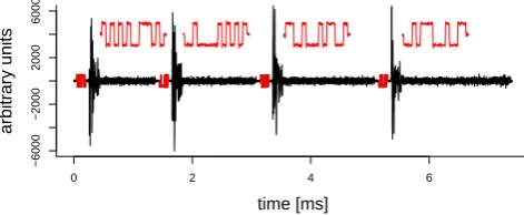
Fig. 1. Raw data of a full transmission cycle from experiment 1. Transmission signals are marked with red color. After each pulse a larger image of the transmission envelope is plotted above the received signal.

To allow data analysis with range resolution better than the transmission pulse length, radar codes (transmission modu-lations) of incoherent scatter radar experiments are usually selected to fulfill certain decoding properties. However, the need of a special decoding method can be removed with lag profile inversion, which allows any phase code to be anal-ysed with desired range-, lag- and time-resolutions. Though the inversion is possible with any phase code or a sequence of codes, the estimation accuracy of an experiment is much dependent on the codes used. When introducing the present lag profile inversion software (Virtanen et al., 2008), the pos-sibility to search for efficient radar codes without taking care of the decoding properties (Vierinen et al., 2008) was men-tioned, but only alternating code (Lehtinen and H¨aggstr¨om, 1987) experiments were used to allow comparison between the two analysis methods. The lag profile inversion analy-sis of short code sequences has been earlier used at the EIS-CAT Svalbard radar by Lehtinen et al. (2002). The exper-iments used in this paper are the first ever utilising a new phase coding techique, which has estimation accuracy com-parable to that of alternating codes, though the code cycle is very short. In this paper code sequences consisting of four different phase coded pulses are used, which is the reason to use the term “code quad” when referring to these codes. The method for evaluating different code sequences is introduced in another paper in this issue (Lehtinen et al., 2008), where the code quads are also compared to other kinds of radar cod-ing techniques.

2 New experiments

In this paper two experiments selected from several test runs performed during the finnish EISCAT campaign on October 2007 are introduced. The first of the experiments, hereafter referred as “experiment 1”, was run with the UHF radar. Its D-region capabilities are mainly limited to the short lags, none of which significantly differs from power profile at

D-Table 1. Phase codes used in the experiments.

15-bit code quad

+ − + − + − + − − + + + − + −

− − + − − − − − + − + − + − +

+ + − − + − − − + − + + − − +

− − + − + + + − − − + − − + +

4-bit weak alternating code

− − + −

− + − −

+ − − +

+ + + +

13-bit Barker code

+ − + − + + − − + + + + +

region altitudes. However, the pulses are sufficiently short for measuring the power profile from quite low ranges.

The second experiment, hereafter referred as “experi-ment 2”, was run with the VHF radar. It provides a large number of useful pulse-to-pulse lags in addition to the short ones. The full code cycle of the experiment contains 16 phase coded pulses with varying bit and pulse lengths. More de-tailed information about the experiments is given in the fol-lowing sections.

2.1 Experiment 1

Experiment 1 utilises one phase code sequence, the 15-bit code quad in Table 1. Bit length of the codes is 10 µs lead-ing to total pulse length of 150 µs. The selected bit length makes the experiment optimal for roughly 1 km target range resolution (Lehtinen, 1989). This does not mean that struc-tures smaller or larger than 1 km could not be seen, because the estimation accuracy drops relatively slowly as the target resolution changes to either direction. The experiment was recorded as raw data with 2 MHz sampling frequency, which theoretically allows analysis with 75 m range resolution.

The four pulses in the code quad are transmitted with un-equal IPPs, i.e. there is a different receiving time after each pulse in the quad. The IPPs, measured from start of a pulse to start of the next one, are 1400, 1700, 2000 and 2300 µs. Real part of raw data from one full code cycle is plotted in Fig. 1.

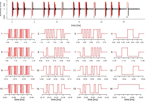
Fig. 2. Top panel: Raw data of a full transmission cycle from experiment 2. Transmission signals are marked with red color. Lower panels: Larger images of the numbered transmission envelopes, notice the differing time scales.

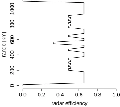
samples with contribution from each range. To make com-parison of different experiment easier, we use the concept of radar efficiency: the number of echo samples from each range is normalized using the total duration of the experi-ment and the maximum duty cycle of the radar so that the largest possible efficiency is 1.0, meaning that the radar duty cycle is fully occupied and all echoes are received. Values smaller than one mean either that the duty cycle is not fully occupied or echoes are lost during subsequent transmissions. The radar efficiency for experiment 1 as a function of range is plotted in Fig. 4.

There are certain technical limitations causing the effi-ciency values clearly smaller than one: The clystron beam must be turned on 40 µs before the start of an actual pulse and there is an upper limit of 12.6% for the beam duty cy-cle. From these numbers we can calculate that the true max-imum RF duty cycle for 150 µs pulses is 10% corresponding the value 0.8 in radar efficiency. In fact the maximum RF duty cycle of the EISCAT UHF radar (12.4%) can only be

achieved with the maximum allowed pulse length (2000 µs). The efficiency value is not constant because some echoes are always lost during the transmissions of the subsequent pulses. This behavior is not a specific weakness of the new experiments, similar deviations from the maximum value would result also if several frequency channels would be used to fill the radar duty cycle.

2.2 Experiment 2

Experiment 2 can be seen as an extended version of experi-ment 1. Its code cycle consists of 16 different phase coded pulses, among which three different bit lengths are used. The code cycle is constructed by combining four sets of four phase coded pulses. The properties of the code sets are listed in Table 2.

2284 I. I. Virtanen et al.: Towards multi-purpose experiments

0.0 0.2 0.4 0.6 0.8 1.0

0

100

200

300

400

500

radar efficiency

range [km]

Fig. 3. Radar efficiency for standard EISCAT UHF experiment “manda”. Here efficiency value 1.0 would mean that the maximum duty cycle of 12.4% is fully used. Though the experiment is anal-ysed up to larger ranges than the length of one IPP, a “dead” range is produced around 300 km from which no echoes are received.

0.0 0.2 0.4 0.6 0.8 1.0

0

200

400

600

800

1000

radar efficiency

range [km]

Fig. 4. Radar efficiency for experiment 1 introduced in this paper.

IPPs are 1104, 1450, 1750, 2740, 1004, 1350, 1650, 2640, 1204, 1550, 1850, 2540, 1304, 1650, 1880 and 2934 µs. Real part of raw data from a full code cycle is plotted in Fig. 2.

According to Lehtinen (1989), the bit lengths of the code sets 1, 2 and 4 are optimal for roughly 200 m, 1 km and 6 km target resolutions, respectively (set 3 is exactly the same as set 2). Moreover, the pulse-to-pulse and fractional lags are supposed to be optimal for target resolution corresponding the shorter bit lengths, as the optimal target resolution is de-termined by the Fourier components of the range ambiguity function (Lehtinen, 1989). The radar efficiencies for each different code and the total efficiency are plotted in Fig. 5. Despite the short IPPs the theoretical range extent of the ex-periment is very large.

0.0 0.2 0.4 0.6 0.8 1.0

0

1000

2000

3000

4000

radar efficiency

range [km]

Fig. 5. Radar efficiency for experiment 2 introduced in this paper. Efficiency of the code with 2 µs (magenta), 10 µs (blue) and 60 µs (red) bits are drawn as separete curves. The black curve is the total efficiency.

Table 2. Code sets used in experiment 2. If Barker codes are used the bit length in fourth column is that of the Barker code.

set number code set sub-bit

Barker code bit length [µs]

set 1 4-bit weak alternating code 13-bit 2

set 2 15-bit code quad – 10

set 3 Same as set 2 – 10

set 4 4-bit weak alternating code – 60

3 Analysis results

Both short lags (shorter than longest pulse length) and D-region pulse-to-pulse lags were inverted from recorded raw data using lag profile inversion software described in (Virta-nen et al., 2008). The resolutions used in the following ex-amples are just one possible choice, the combination of raw data and lag profile inversion gives the user a freedom to se-lect the resolutions after running the experiment and also to analyse the same data with different resolutions.

● ● ● ● ●●● ●●● ●●● ●● ●●●● ●●●●●●●● ● ● ●● ● ● ● ● ● ● ● ● ● ● ●

10.0 10.5 11.0 11.5 12.0

100 150 200 250 300 Electron Density

Log(Ne) [m −−3_]

Height [km] ● ● ● ● ● ● ● ● ● ● ● ● ● ● ●●● ●● ● ●● ● ●● ● ●●● ●●● ● ● ● ●● ● ● ● ● ● ● ● ● ● ● ●

0 500 1000 1500

100 150 200 250 300 Ion Temperature [K] Height [km] ● ● ● ● ● ● ● ● ● ● ● ● ● ● ● ● ●●● ●●●●●●● ●●● ●●● ● ●● ● ●● ● ● ● ● ● ● ● ● ● ●

0 500 1000 1500 2000 2500 3000

100 150 200 250 300 Electron Temperature [K] Height [km] ● ● ● ● ● ● ● ● ● ● ● ● ● ● ●● ● ● ●●●●●●●●●● ● ● ● ● ● ● ● ● ● ● ● ● ● ● ● ● ● ● ● ●

−200 −100 0 100 200

100 150 200 250 300 Ion Velocity

[ms−−1

]

Height [km]

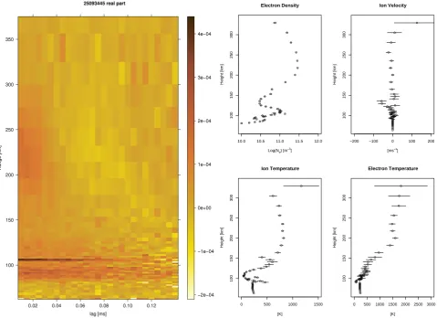
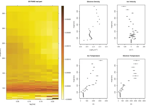
Fig. 6. Analysis results of experiment 1 from 18 October 2007 10:24 UT. Left panel: Real part of ACF in arbitrary units. Time resolution is 5 s and range resolution varies from 1.5 km in D- and lower E-regions to 50 km above F-region peak. Right panel: Plasma parameters with 1 min integration time. The horisontal lines are 68% confidence intervals. Model values are used for ion mass and collision frequency at all altitudes, for ion temperature and electron to ion temperature ratio below 90 km and ion velocity is set to zero below 90 km. Electron density is not calibrated.

of a four-parameter fit with 1 min time resolution is plotted in right panel of Fig. 6.

An attempt was also made to invert D-region pulse-to-pulse lags from the data, but as assumed the echoes do not correlate long enough for reasonable pulse-to-pulse measure-ments. (This is usually the case with UHF experimeasure-ments. A VHF version of this experiment is expected to produce use-ful pulse-to-pulse data, but the VHF version was not run this time.) Anyhow, the D-region power profile was successfully measured.

Experiment 2 was analysed with the same range- and time-resolutions as experiment one. Because the shortest bit length in the experiment was only 2 µs, the data can not be decimated to longer sampling interval than this. On the other hand, because the ACFs of the VHF radar are about four times as long as those of the UHF radar, even lower lag res-olution than that used for experiment 1 could be used. For

these reasons several fractional lags were included in each main lag to produce the 25 µs lag resolution seen in the left panel of Fig. 7. A similar four-parameter fit as performed for experiment 1 was also made for the experiment 2, the re-sult of the parameter fit is seen in the right panel of Fig. 7. Though the lag profiles were successfully inverted, it is evi-dent that the pulses in experiment 2 were too short for mea-suring ion and electron temperatures at E and lower F re-gions. From the ACF plot it is seen that below 200 km even the first zero of the ACF is not meat, which leads to doubtful fit results for the temperatures.

2286 I. I. Virtanen et al.: Towards multi-purpose experiments ● ● ● ● ● ●● ● ● ● ● ● ● ● ● ● ●●● ●● ● ● ● ● ● ● ● ● ● ● ●

10.0 10.5 11.0 11.5 12.0

100 150 200 250 300 Electron Density

Log(Ne) [m−− 3 ] Height [km] ● ● ● ● ● ● ● ● ● ● ● ● ● ● ●●●●●●●●● ●● ● ● ● ● ● ● ● ● ● ● ●

0 500 1000 1500 2000

100 150 200 250 300 Ion Temperature [K] Height [km] ● ● ● ● ● ● ● ● ● ● ● ● ● ●● ●●● ● ● ● ● ●● ●● ● ● ● ● ● ● ● ● ● ●

0 500 1000 1500 2000 2500 3000

100 150 200 250 300 Electron Temperature [K] Height [km] ● ● ● ● ● ● ● ● ● ● ●● ● ●● ● ● ● ● ● ●● ● ● ● ● ● ● ● ● ● ● ● ● ● ●

−200 −100 0 100 200

100 150 200 250 300 Ion Velocity

[ms−−1

]

Height [km]

Fig. 7. Analysis results of experiment 2 from 19 October 2007 09:28 UT. Left panel: Real part of ACF in arbitrary units. Time resolution is 5 s and range resolution varies from 3 km in D- and lower E-regions to 50 km above F-region peak. Right panel: Plasma parameters with 1 min time resolution. The horisontal lines are 68% confidence intervals. Model values are used for ion mass and collision frequency at all altitudes, for ion temperature below 100 km, for electron to ion temperature ratio below 150 km and ion velocity is set to zero below 90 km. Due to insufficiently short pulses of the experiment the fit results for temperatures may not be reliable. Electron density is not calibrated.

lags inside each slide were combined in one lag profile, i.e. the final lag resolution of the analysis is 1 ms. The analy-sis program tests all lag values and automatically drops off those ones which do not have any non-zero parts in range ambiguity function. In this way different lag values may get different estimation accuracies as the lag profiles are combi-nations of varying number of fractional lags, which is readily seen in the variances of the inversion results. For the user this kind of analysis is particularly easy, as no information of the actual IPPs is needed.

We want to specially emphasize the fact that all kinds of lagged products are included in the inversion, especially also those resulting from correlation between the Barker coded alternating codes and the plain alternating codes, as well as the products resulting from correlation between the Barker coded alternating codes and the 15-bit code quads. Also the fractional lags between the 15-bit code quads contribute

significantly to the high-resolution estimates. Moreover, of course even the not-so-fractional (close to full) lags con-tribute, even if their ambiguity functions consist of bits wider than the desired resolution. Everything is automatically in-cluded, correctly weighted, by the inversion process. All this is omitted in a standard type of experiment, where different code sequences are on different frequencies and they cannot be correlated with each other.

anything that could be directly used for comparisons with other experiments. Numerical studies of the variance behav-ior much similar to those presented in Lehtinen et al. (2008) could be performed using lag profile inversion. This kind of analysis will be important when designing future experi-ments, but in this paper we settle on demonstrating that we are able to analyse the new experiments. If the phase codes used would perform perfectly with the unequal IPPs and if the assumption of small signal to noise ratio is justified, the ratio of best attainable accuracy and that attained from the new experiments would follow the radar efficiency curves in Figs. 4 and 5. Here one should notice that the efficiency 1.0 is very difficult to achieve in practical experiments as men-tioned in Sect. 2.1.

4 Resources needed for real-time lag profile inversion

The experiments used in this paper were both analysed in real-time using lag profile inversion, but with too low res-olutions to be used for storing the data. The analysis task was shared with eight processors without any special par-allel processing – the parpar-allelization was accomplished at the UNIX command line level by generating independent command-line analysis processes accessing different pieces of data. These commands were generated automatically by R scripts (R Development Core Team, 2007), which was also used for visualization and user interface. The analysis speed was also increased by calculating averages of raw lag profiles before the inversion, which is not the most accurate way of performing the analysis. The results in this paper were later calculated without the averaging. Here some numbers are shown of the computing resources needed for high-resolution lag profile inversion in real-time.

The resolutions needed for the stored lag profiles are very much dependent on the experiment and its target. In the fol-lowing calculations it is assumed that an integration time of 2 s is always used. Then range extent, number of range gates and data decimation are varied. The number of floating point operations needed for the analysis (FLOP count) and the CPU time used by the current analysis computer (8×3 GHz Eight-Core Intel Xeon, 16 GB 667 MHz DDR2 FB-DIMM, Apple Mac Pro) are measured. An auto-vectorized 64-bit ex-ecutable using 32-bit floating point precision was built with Intel Fortran version 10.0.

The factors that can affect the FLOP count and CPU time are assumed to be the amount of decimation of the amplitude-domain data, the number of range gates and the range ex-tent of the analysis. Also the experiment timing has effect to the analysis time, because the FLIPS package (Orisp¨a¨a and Lehtinen, 20081) can solve the problem faster if there are many zeros in the beginning or end of the theory matrix rows. In this sense having several pulses simultaneously in

1_{Orisp¨a¨a, M. and Lehtinen, M. S.: Fortran Linear Inverse}

Prob-lem Solver (FLIPS), unpublished manuscript, 2008.

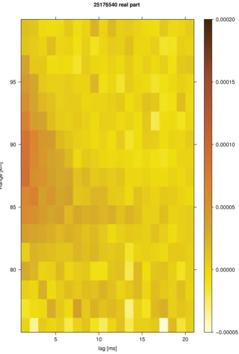
Fig. 8. Real parts of some D-region pulse-to-pulse lag profiles from experiment 2 19 October 2007 09:28 UT. The time resolution is 1 min, lag resolution 1 ms and range resolution 1.5 km. The ACF is in arbitrary units, but in same units as the ACF in Fig. 7.

ionosphere is not optimal situation for lag profile inversion, since it leads to theory matrix rows with only few zeros, if any, in both ends.

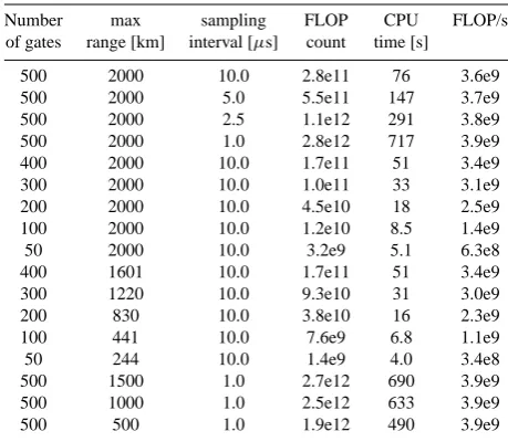
In Table 3 there are some numbers from test runs with the experiment 2 introduced in this paper. As high range resolu-tions (of the order of 100 m) are sometimes needed in lower ranges, the data can not be decimated much when analysed for storage purposes. On the fifth row is the combination of the nearest values that could be used in routine storage. The other numbers are calculated to see how the software behaves as the parameters are varied.

2288 I. I. Virtanen et al.: Towards multi-purpose experiments

Table 3. Computing power needed for selected resolutions. All numbers are for one lag profile starting from 50 km range. Integra-tion time is 2 s. The CPU times are for one core of an 8×3 GHz Eight-Core Intel Xeon desktop computer, 16 GB 667 MHz DDR2 FB-DIMM (Apple Mac Pro). The theoretically maximum possible FLOP/s rate of such a core is 4 times the CPU frequency assuming the vector SIMD SSE unit can operate at full speed making four 32-bit vector floating point operations each clock cycle. Thus the theoretical speed being 1.6e10 FLOP/s and the actual speed being about a quarter of that in many cases can be considered very satis-factory.

Number max sampling FLOP CPU FLOP/s

of gates range [km] interval [µs] count time [s]

500 2000 10.0 2.8e11 76 3.6e9

500 2000 5.0 5.5e11 147 3.7e9

500 2000 2.5 1.1e12 291 3.8e9

500 2000 1.0 2.8e12 717 3.9e9

400 2000 10.0 1.7e11 51 3.4e9

300 2000 10.0 1.0e11 33 3.1e9

200 2000 10.0 4.5e10 18 2.5e9

100 2000 10.0 1.2e10 8.5 1.4e9

50 2000 10.0 3.2e9 5.1 6.3e8

400 1601 10.0 1.7e11 51 3.4e9

300 1220 10.0 9.3e10 31 3.0e9

200 830 10.0 3.8e10 16 2.3e9

100 441 10.0 7.6e9 6.8 1.1e9

50 244 10.0 1.4e9 4.0 3.4e8

500 1500 1.0 2.7e12 690 3.9e9

500 1000 1.0 2.5e12 633 3.9e9

500 500 1.0 1.9e12 490 3.9e9

If raw data is stored and real-time analysis is used only for monitoring the ionosphere, much larger range gates and a smaller number of lags can be used. Using the table we can calculate that 20 lag profiles with 100 range gates, 1.5 km maximum resolution and 2 s integration time requires about 240 GFLOPs. This is accomplished in 170 s with one proces-sor. In other words, this kind of real-time monitoring requires 120 GFLOP/s which can be achieved using about 85 cores or eleven computers. In many cases even much smaller number of range gates is enough for monitoring purposes.

It may seem that analysing the recorded raw data at higher resolutions would be a huge effort. Here one needs to notice that if lag profiles are stored they need to have high resolu-tion, but this is only to be prepared for unusual ionospheric conditions. Raw data contains the necessary information for high-resolution analysis, but for most parts of the data much lower resolutions are sufficient. The small fraction of the data that needs high-resolution analysis can usually be selected from the lower resolution results thus avoiding unnecessary calculations.

5 Storage resources

In the previous section we estimated the computational re-sources necessary for real-time inversion of lag profile data and found that while it is perfectly possible to do real-time inversion for monitoring purposes, inversion for resolutions good enough to facilitate use of inverted lag profile data for further analysis requires very much in terms of computa-tional power. While this kind of computacomputa-tional power might still be a reasonable requirement for a future incoherent scat-ter facility, we feel it is useful to consider storage of raw (uncorrelated) amplitude-domain data instead of the storage of lag profiles.

The analysis in this paper is based on baseband detected complex data. The sampling frequency was 2 MHz facili-tating 75 m range resolution throughout the ionosphere and arbitrarily high time resolution. The possible lag values are limited by the selected pulse lengths and IPPs, but within these limits a lag resolution of 0.5 µs can be achieved. On the other hand, by including several lag profiles in same inver-sion problem arbitrarily low lag resolutions are also possible without losing the high range resolution. In addition there is no limitations for the longest lag. We have routinely used this kind of data storage for finnish special experiments and can presently store 4 Terabytes of data on a cheap commer-cial RAID disk system, enough for 138 h of raw amplitude-domain data. The 2 MHz sampling frequency is not enough for recording the plasma lines, but the plasma line informa-tion is lost in standard lag profile storage also. To maintain the plasma line information in the data one can either in-crease the sampling frequency or analyse the plasma lines as separate process in real time using other analysis methods.

6 Conclusions

In this paper we have demonstrated how the transmission pulses of incoherent scatter radar experiments can be ar-ranged in a way that allows lag profile analysis with a large range coverage though the pulses are transmitted with short inter pulse periods. The data analysis of this kind of an ex-periment is also demonstrated with real exex-perimental data. Though the lag profile inversion part of the analysis was suc-cessful, the fit of ion and electron temperatures was not very successful with experiment 2. The problem is easy to solve by including longer pulses in the experiment to allow long enough lags to be inverted. The experiment optimisation in the form of carefully evaluating and minimising the vari-ances of the inverted lag profiles is the natural next step in this work.

flexible storage format for future IS radars. Also, in terms of actual hardware, saving baseband data is trivial with off-the-shelf equipment. The full (ion line) bandwidth of a radar signal generates about the same data bandwidth as a standard HD video stream at the time of writing this article.

Acknowledgements. The EISCAT measurements were made with

special programme time granted for Finland. EISCAT is an inter-national assosiation supported by China (CRIRP), Finland (SA), Germany (DFG), Japan (STEL and NIPR), Norway (NFR), Swe-den (VR) and United Kingdom (PPARC). This work was supported by the Academy of Finland (application number 213476, Finnish Programme for Centres of Excellence in Research 2006-2011; ap-plication number 43988, EISCAT Data Analysis and Research) and by the Finnish Graduate School in Astronomy and Space Physics.

Topical Editor K. Kauristie thanks I. H¨aggstr¨om and another anonymous referee

References

Lehtinen, M., Markkanen, J., V¨a¨an¨anen, A., Huuskonen, A., Damtie, B., Nygr´en, T., and Rahkola, J.: A new incoherent scat-ter technique in the EISCAT Svalbard Radar, Radio Sci., 37, 3–1, doi:10.1029/2001RS002518, 2002.

Lehtinen, M. S.: On optimization of incoherent scatter measure-ments, Adv. Space Res., 9, 133–141, doi:10.1016/0273-1177(89) 90351-7, 1989.

Lehtinen, M. S. and H¨aggstr¨om, I.: A new modulation principle for incoherent scatter measurements, Radio Sci., 22, 625–634, 1987. Lehtinen, M. S., Virtanen, I. I., and Vierinen, J.: Fast comparison of IS radar code sequences for lag profile inversion, Ann. Geophys., 26, 2291–2301, 2008,

http://www.ann-geophys.net/26/2291/2008/.

R Development Core Team: R: A Language and Environment for Statistical Computing, R Foundation for Statistical Computing, Vienna, Austria, http://www.R-project.org, ISBN 3-900051-07-0, 2007.

Turunen, T., Westman, A., H¨aggstr¨om, I., and Wannberg, G.: High resolution general purpose D-layer experiment for EISCAT in-coherent scatter radars using selected set of random codes, Ann. Geophys., 20, 1469–1477, 2002,

http://www.ann-geophys.net/20/1469/2002/.

Vierinen, J., Lehtinen, M. S., Orisp¨a¨a, M., and Virtanen, I. I.: Trans-mission code optimization method for incoherent scatter radar, Ann. Geophys., accepted, 2008.

Virtanen, I. I., Lehtinen, M. S., Nygr´en, T., Orisp¨a¨a, M., and Vieri-nen, J.: Lag profile inversion method for EISCAT data analysis, Ann. Geophys., 26, 571–581, 2008,