Efficient Techniques for Simulation of Interest Rate Models Involving Non-Linear Stochastic Differential Equations

Efficient Techniques for Simulation of Interest Rate

Models Involving Non-Linear Stochastic Differential

Equations

by

Leif B. G. Andersen

Vice President, Research

General Re Financial Products Corp.

630 Fifth Avenue, Suite 450

New York, NY 10111

(212)-307-2339

<[email protected]>

Preliminary Version

Efficient Techniques for Simulation of Interest Rate Models involving

Non-Linear Stochastic Differential Equations

Abstract

Efficient Techniques for Simulation of Interest Rate Models involving

Non-Linear Stochastic Differential Equations

1. Introduction

Driven by the increasing sophistication and competitiveness of the financial markets, much recent finance research emphasizes that theoretical models be "realistic", i.e. closely reflect observable market behavior. Whereas the structure of most classical models has been specified primarily with analytical tractability in mind, many new models deliberately sacrifice such tractability for a closer fit to the market. The lack of tractability, however, makes the practical usage of such models reliant upon the development of efficient numerical schemes. Indeed, the finance literature has recently seen an abundance of ingenious schemes designed either to support complicated, non-linear models or to provide automatic calibration to observable prices. Most of these schemes are based on binomial or trinomial discretizations of either the underlying stochastic processes or the fundamental no-arbitrage PDE. Examples from the interest rate markets include Jamshidian (1991), Hull and White (1990a, 1994a-b), Black, Derman and Toy (1990), Ho and Lee (1986), Jensen & Nielsen (1991) just to name a few. In equity markets Wilmott, Dewynne and Howison (1993), extending the work of Brennan and Schwartz (1978), have illustrated how many types of exotic options can be priced efficiently in either finite difference or finite element lattices. Recently, Dupire (1993, 1994), Derman and Kani (1994), Rubinstein (1994), and Andersen and Brotherton-Ratcliffe (1995) have shown how to use forward induction principles to extend lattice and finite difference models to incorporate the effects of the so-called "volatility smile" in options markets.

stochastic factors1. As complexity of traded instruments has grown, Monte Carlo techniques have become increasingly important, a trend that is likely to continue in the future. This is particularly true in the fixed income markets, where multiple factors and path-dependency are embedded in a wide variety of new structured or mortgage-based contracts. Despite its increasing importance and wide applicability, the Monte Carlo method has received much less attention in the literature than lattice models. One reason for this is, of course, the low order of convergence (O N( −1 2/ )) which tends to make practical usage painfully slow. Recent research, however, suggests that application of results from the field of high-dimensional integration can, under certain circumstances, improve this convergence rate significantly. As shown in Brotherton-Ratcliffe (1994a-b), Joy (1994), and Paskov (1994), replacing the traditional pseudo-random number generators by low-discrepancy quasi-random sequences can lead to significant improvements in the computational effort required to value a wide array of path-dependent options and CMOs. Further, by applying a martingale control variate technique to option pricing, Clewlow and Carverhill (1994) report significant improvements over traditional variance reduction methods2. Another line of research has focused on extending the Monte Carlo technique to pricing problems that were previously considered beyond the capabilities of the method. Tilley (1993) and, more recently, Broadie and Glasserman (1994) have shown how, in principle, Monte Carlo simulation can be used to price American-style equity options. Andersen (1996), and Andersen and Brotherton-Ratcliffe (1996) illustrate how the Monte Carlo method can successfully be applied to the pricing of lookback and barrier options with continuous or high-frequency sampling of the underlying asset process.

Almost all recent research on Monte Carlo methods share the common assumption that the underlying asset process is simple deterministic geometric Brownian motion -- a process class characterized by a linear stochastic differential equation (SDE) that permits a closed-form solution. Given the price at time t, St, of an asset that follows geometric Brownian

Ss St u u du z u du

t s

t s

= exp

I

I

2

2 2

(1)

where ~z is a standard Gaussian variable, and the deterministic functions of time µ( )t and σ( )t are the drift and volatility of S, respectively. In the case of geometric Brownian

motion, simulation of asset-paths is thus essentially a matter of repeated application of (1). In interest rate modeling, which will be the main focus of the present paper, it is, however, highly questionable whether we can assume that market dynamics are governed by simple linear SDEs. Many popular interest rate models thus involve highly non-linear SDEs, including those of Pearson and Sun (1990), Cox (1975), Black, Derman and Toy (1990), and Cox, Ingersoll and Ross (1985)3. Empirical studies by, among others, Das (1993), Chan

et al (1992), and Apabhai et al (1994) confirm the non-linearity of interest rate SDEs4.

In this paper, we will investigate the application of techniques from both Monte Carlo theory and the field of stochastic numerical methods to an interest rate setting. In particular, we will illustrate how careful application of high-order simulation schemes combined with SDE- and Monte Carlo-based variance reduction techniques can lead to significant improvements in convergence of interest rate models. For purposes of exposition, we will limit our discussion to one-factor short rate models; most of the results and general techniques can easily be extended to the case of multiple factors (as in Brennan and Schwartz (1982)) and should also prove useful for forward rate models (as in Heath, Jarrow and Morton (1992)). Further, we will focus most of our discussion to the fundamental problem of determining bond prices from given values of the short rate. As in practice all interest rate contingent claims depend on some, possibly path dependent, function of one or more bond prices (rather than the instantaneous short rate), the capability of quickly extracting accurate bond prices is a prerequisite for simulation of more complicated contingent claims. Throughout the paper we will use the Cox, Ingersoll and Ross (1985) square-root diffusion model to illustrate key results. This model is sufficiently complicated to illustrate the fundamental problems of simulating non-linear SDEs, yet permits a closed-form bond-pricing solution and hence allows for monitoring and testing of simulation results.

2. Setup and Model Assumptions

We consider a frictionless intertemporal economy with a bounded trading horizon [ , ]t0 τ ,

t0 being the present and τ some arbitrary, fixed future time. As usual, we represent

uncertainty by a probability space ( , , )Ω F P where Ω is the set of possible states, F is a σ-field of subsets of Ω, and P is a (real world) probability measure. We will limit our discussions to models where the stochastic dynamics are driven by a single Brownian motion {W t$t, ∈[ , ]}t0 τ . Information flow in the economy is represented by the (augmented)

filtration {ℑ ∈t,t [ , ]}t0 τ generated by W$ and satisfying ℑ =τ F. As always, we assume

that ℑ_t meets the usual conditions, i.e. is right-continuous and contains the null-sets of P.

To characterize the term structure of risk-free interest rates, we let5 the strictly positive, adapted process P t T( , ),t0≤ ≤ ≤t T τ denote the time t price of a bond that matures at time T with certain payout P T T( , )=$1. As discussed in Harrison and Kreps (1979), under technical conditions6 there are no arbitrage opportunities if and only if there exists a probability measure Q, equivalent to P, under which the expected instantaneous rate of return on any discount bond equals the risk-free rate. Q is frequently referred to as the "risk-neutral" probability measure. Under Q, we will assume that the dynamics of the yield curve can be described by a one-factor diffusion process in the instantaneous short rate r taking values in a subset D of ℜ:

drt=µr( , )r t dtt +σr( , )r t dWt t (2)

where {W tt, ∈[ , ]}t0 τ is a Brownian motion under Q and where µ σr, r:D×[ , ]t0 τ → ℜ

have sufficient regularity to ensure the existence of a unique solution to (2) (see for example Arnold (1992), chapter 6)7. In most cases D will be the set of all non-negative real numbers ℜ+, although some (Gaussian) models have D= ℜ.

drt=[ ( )c t1 +c t r2( )t+c t r3( ) ln ]t r dtt +[ ( )k t1 +k t r2( ) ]t γdWt (3)

for constant γ and deterministic coefficients c1, c2, c3, k1, k2: [ , ]t0 τ → ℜ. In this

paper, two special cases of (3) will be of special importance, namely the Cox, Ingersoll,

and Ross (CIR) (1985) model (c3=0, k1=0, γ =0 5. ):

drt=a b r dt( − t) +σ r dWt t (4)

and the Vasicek (1977) model (c3=0, k2=0, γ =10. ):

drt=α β( −r dtt) +κdWt (5)

for positive constants8 a, b, σ , α , β, and κ. In the CIR model, the distribution of the short rate can be shown to be non-central chi-square with mean and variance

CIR:

EQ r rs t r et b e s t

a s t a s t

( | )= − (−)+ (1− − (−)), ≥ (6a)

V r r r

a e e

b

a e s t

Q

s t t

a s t a s t a s t

[ | ]= σ ( − ( −)− − ( −))+ σ ( − − ( −)) , ≥

2

2 2 2

2 1 (6b)

In the Vasicek model, the short rate is Gaussian with moments

Vasicek:

EQ r rs t r et e s t

s t s t

( | )= −α(−)+β(1− −α(−)), ≥ (7a)

VQ r rs t e s t

s t

[ | ]=κ ( − − ( −)), ≥

α α

2 2

2 1 (7b)

model is clearly a problem; due to its analytical tractability, the Vasicek model is nevertheless quite popular in the literature.

In most applications, we are interested in determining the value of discount bonds given the process dynamics in (2). As shown in Harrison and Kreps (1979), discount bond prices are given by the risk-neutral conditional expectation

P t T EQ r duu t E r du

t T

t Q

u t

T

( , )=

!

I

"

$#

_!

I

"

_$#

where we have introduced the notation Et E

Q Q

t

[ ]⋅ = [ |⋅ ℑ]. For later uses, we note that (8) alternatively can be written

P t T Et I

Q T

( , )= [ ] (9a)

where I is given by the SDE

dIs= −r I dss s , It=1, t0≤ ≤ ≤t s τ (9b)

CIR:

P t T_{( , )}= A t T e_{( , )} −r B t Tt ( , ) ₍₁₀₎

A t T e

a e

a T t T t ab ( , ) ( )( ) ( )( )/ ( ) / = + − +

!

"

$#

B t T e

a e T t T t ( , ) ( ) ( )( ) ( ) ( ) = − + − + − − 2 1 1 2 η η η η

η= a2+2σ2

Vasicek:

P t T_{( , )}=C t T e_{( , )} −r D t Tt ( , ) ₍₁₁₎

D t T e

T t

( , )

( )

= −1 −α − α

C t T( , )=exp

!

"

$#

κ α 2 2 2 2 2 2 4

3. Discretization Schemes for Simulation of Discount Bond Prices

3.1. The General Case

To develop schemes for the evaluation of the bond pricing equation (8) or, equivalently, (9a-b), we consider the vector SDE (under Q)

d r I

r t r I dt

r t

dW t t r const D I

t t

r t t t

r t

t t t

−

0 0 0 0 1

(12)

r I

r I

r t r I s t

r t

W W R t t s

s s t t r t t t r t s t

0 1 0

r

(13)

where the remainder vector Rr1 consists of multiple stochastic integrals of second order.

The second-order Ito-Taylor expansion of (12) takes the form

r I

r I

r t r I s t

r t

W W

L r t I r r t

s t L r t W W s t

L r t I r t

s s t t r t t t r t s t r t t t r t

r t

s t

r t t r t

2 1 2

1

4

9

4

9

r t

s t s t

0

2

0

σ

₁

₆

(14)

where the remainder Rr2 involves third-order stochastic integrals. In (14), we have

introduced the operators

L

t r r r r L r r

0 2 2 2 1 1 2 = ∂ + ⋅ + ⋅ = ⋅ ∂ µ ∂ ∂ σ ∂ ∂ σ ∂ ∂

( ) ( ) ; ( ) (15)

and a new Gaussian process11 Vt given by Et V V Q

s t

[ − ]=0, Et V V s t

Q s t

[( − ) ]2 = −( ) /3 3,

and Et V V W W s t

Q

s t s t

[( − )( − )]= −( ) /2 2.

To simulate a single path of r and I over the interval [ , ]t T0 , we discretize the time interval

First-order Taylor (Euler):

$ $_{( $ ) ,}

Ii+1=Ii1−riδ (16a)

$ $ ($, ) ($, )~ ,

, ,..., , $ , $

r r r t i r t i z

i K r r I

i i r i r i i

t

+ = + + + + +

= − = =

1 0 0 1

0 0

0 1 1 ₀ 1

µ δ δ σ δ δ

(16b)

Second-order Taylor (Milstein):

$ $ _{$ $ ($, ) ($, )~ ,}

Ii+1=Ii

2 0 2 0 1 1 1 2 1 2

δ

4

9

$ $ ($, ) ($, ) ($, )~

($, ) ($, ) ~ ($, )

($, )~ , , ,..., , $ , $

r r r t i L r t i r t i z

L r t i L r t i z L r t i

L r t i z i K r r I

i i r i r i r i i

r i r i i r i

r i i t

+ + + + = +

0 0 1

1 0 0 0 1 0 0 2 1 0 1 2 0 1 2 1 2 1 2 1

2 0 1 1 0

µ δ σ δ δ σ δ δ

µ δ σ δ δ δ µ δ δ

σ δ δ

4

9

0=1

(17b)

In (16a-b) and (17a-b) we have set Wi+1−Wi=~zi+1 δ , where ~ , ~ ,..., ~z z1 2 zK is an

independent sequence of standard Gaussian variables, ~zi∈N( , )0 1 . In (17a-b) we have

further set Vi+1− =Vi ~zi+1δ δ /2; this simplification can be shown to be valid for the

purpose of evaluation expectations of the joint vector processes (12) (which is what we are interested in here); see Kloeden and Platen (1992), chapter 14 for a proof. In the literature, the first-order Taylor approximation (16a-b) is known as the Euler scheme, whereas (17a-b) is an extended version of the Milstein scheme.

If we apply (16a-b) or (17a-b) to generate N sample values of the process I$ at time T,

$ _,$ _,...,$

IK IK IK N

1 2

$_{( , )} $

P t T

N IK

j j

N

0

1

1

=

=

∑

To analyze the quality of the estimate P t T$( , )0 , it is convenient to decompose the total

mean error

$ $( , ) ( , )

e=P t T0 −P t T0 (19)

into two components, a systematic error esys and a statistical error e$stat:

$ $

e=esys+estat (20)

where esys is a constant

esys Et e E P t T P t T E I P t T

Q t Q

t Q

K

= ₀[$]= ₀[$( , )]0 − ( , )0 = ₀[$ ]− ( , )0 (21)

and e$stat is a random variable with mean Et e Q

stat

0[$ ]=0 and variance

V e V e V P t T

NV I

t Q

stat t Q

t Q

t Q

K

0 0 0 0 0

1

[$ ]= [$]= [$( , )]= [$ ] (22)

Under certain smoothness and regularity conditions on µ_r and σ_r, it can be shown that both the Euler and Milstein schemes have the property that esys→0 for δ→0 ; however,

the speed at which esys approaches zero depends on which scheme is used. More precisely,

one can show (Kloeden and Platen (1992), p. 473-74) that the following inequalities hold

Euler Scheme: esys ≤C1δ (23a)

Milstein Scheme: esys ≤C2

2

where C1 and C2 are positive real constants independent of the step-size δ. Based on the

exponent of δ in the above inequalities we say that the Euler and Milstein scheme

converge weakly with order 1 and 2, respectively .

Schemes with weak convergence orders greater than 2 can, in principle, be constructed from high-order Ito-Taylor expansions of (12). Unfortunately, such expansions generally lead to non-trivial multiple stochastic integrals which frequently require the usage of quite complicated approximation techniques. An attractive alternative to the truncated Taylor series is Richardson extrapolation which essentially allows us to construct high-order schemes by combining results from low-order schemes. Suppose for example that we use the Milstein scheme (17a-b) to construct two bond price estimates, P t T$_δ( , )0 and

$ _{( , )}

P2δ t T0 , for step-sizes δ and 2δ, respectively. Under technical conditions on µr and

σr, an error expansion result by Talay and Tubaro (1990) can be used to show that the

combination

$ _{, ( , )} $_{( , )} $ _{( , )}

PRδ t T0 P t Tδ 0 P2δ t T0

1

3 4

=

4

9

converges with weak order 3. As in the deterministic case, Richardson extrapolation works

through cancellation of leading order error terms.

3.2 Discretization and Test of the CIR Model

Applying the general formulas (16a-b) and (17a-b) to the CIR process12 (4) yields the following discretization schemes:

Euler Scheme:

$ $_{( $ ) ,}

Ii+1=Ii1−riδ (25a)

$ $ ( $) |$|~ , , ,..., , $ , $

ri+1= +ri a b r− i δ σ+ r zi i+1 δ i=0 1 K−1 r0=rt₀ I0=1 (25b)

Milstein Scheme:

$ $ _{$ $ ( $) |$|~ ,}

Ii+1=Ii

2 2 1 1 1 2 1 2

δ

4

9

$ $ ( $) |$|~

|$| ( $) |$|

~ _{( $)}

~ _{, , ,..., , $ , $}

r r a b r r z

r a b r r a z a b r

z i K r r I

i i i i i

i

i i i i

i t + + + + = +

4 0 1 1 0 1

σ δ σ δ

σ σ _{δ δ δ}

σ _δ

(26b)

As the discretized CIR process -- unlike its continuous-time equivalent -- has a non-zero probability of generating negative short rates, notice that we have taken the precaution of using absolute values of r$i in all square-root operations in (25a-b) and (26a-b). Since the

CIR model permits a closed-form bond pricing equation (see (10)), we can, in principle, test the convergence properties of (25a-b) and (26a-b). One complicating factor in convergence tests using a finite number of simulation paths is the presence of the statistical error term e$stat (see (22)) which necessitates construction of confidence intervals around

the total number N of path simulations into B batches of S simulations each, N =SB. Provided that S is sufficiently large (say, larger than 20), the Central Limit Theorem implies that the batch errors will be approximately Gaussian. Using the standard Student T-test we can then use the sample variance

$

( )

$ $

V

B B B P P

B k k

k B k

B

=

− −

∑

∑

1

2 1

2

1

of the B batch averages P P$1,$2,...,P$B to construct the necessary confidence intervals around

the total mean error e$. For example, the 90% confidence interval for e$ has the form

$ .

e±c0 9, c0 9. =t0 9. ,B−1 V$B/B where the multiplier t0 9. ,B−1 is the two-tailed 90th percentile

of a Student T-distribution with B-1 degrees of freedom. Some examples of t0 9. ,B−1 include: t0 9 9. , =183. , t0 9 99. , =166. , and t0 9 999. , =165. .

In Table 1 below, we have listed simulation results for a 2-year discount bond assuming model parameters13 of a=0 4. , b=01. , σ =01. , and an initial short rate of r0=0 06. . The

table covers both the Euler scheme (25a-b), the Milstein scheme (26a-b), and the extrapolated third-order scheme (24). In an attempt to minimize the effects of the statistical error e$stat in (21), we have set N=1,000,000 ( S= =B 1,000 ). The table contains the 90%

confidence intervals of the absolute error, e$±c0 9. , as well as a "worst-case" absolute error,

defined by

$ $ _. , $ _.

e_wc = MAX e

2

7

For comparisons of computational efficiency, the table lists calculation times Tcomp (in

Crude Monte Carlo Simulation Results for CIR Model 2-Year Discount Bond, Theoretical Value = 0.8655244

N=1,000,000;S=1,000;B=1,000

a=0 4. ,b=01. ,σ=01. ,r₀=0 06.

K 1 2 4 8 16 32 64 128 256

δ 2 1 0.5 0.25 0.125 0.0625 0.03125 0.01563 0.00781

log ( )2 δ 1.00 0.00 -1.00 -2.00 -3.00 -4.00 -5.00 -6.00 -7.00

Euler ê 1.45E-2 3.06E-3 9.93E-4 3.62E-4 1.79E-4 7.60E-5 4.15E-5 4.53E-5 5.15E-5 log |2e$| -6.11 -8.35 -9.98 -11.43 -12.45 -13.68 -14.56 -14.43 -14.25

$

V_B 0 7.49E-4 7.97E-4 8.39E-4 8.63E-4 8.50E-4 8.43E-4 8.53E-4 8.46E-4 c0 9. 0 3.91E-5 4.16E-5 4.38E-5 4.50E-5 4.44E-5 4.40E-5 4.45E-5 4.42E-5

|e$ |wc 1.45E-2 3.10E-3 1.03E-3 4.05E-4 2.24E-4 1.20E-4 8.54E-5 8.98E-5 9.56E-5 log |2e$ |wc -6.11 -8.33 -9.92 -11.27 -12.12 -13.02 -13.51 -13.44 -13.35

T_comp 10.90 19.33 35.42 68.87 137.11 274.12 537.30 1065.74 2130.95 log (2Tcomp) 3.45 4.27 5.15 6.11 7.10 8.10 9.07 10.06 11.06

Mil- ê -1.03E-2 -1.88E-3 -3.81E-4 -1.07E-4 -8.36E-6 -5.54E-6 2.88E-6 2.73E-5 4.28E-5

stein log |2e$| -6.60 -9.05 -11.36 -13.19 -16.87 -17.46 -18.40 -15.16 -14.51 $

VB

1.08E-3 9.08E-4 8.65E-4 8.69E-4 8.78E-4 8.56E-4 8.46E-4 8.55E-4 8.47E-4

c0 9. 5.62E-5 4.74E-5 4.51E-5 4.54E-5 4.58E-5 4.47E-5 4.41E-5 4.46E-5 4.42E-5

|e$ |wc 1.03E-2 1.93E-3 4.26E-4 1.53E-4 5.42E-5 5.02E-5 4.70E-5 7.19E-5 8.70E-5 log |2e$ |wc -6.60 -9.02 -11.20 -12.68 -14.17 -14.28 -14.38 -13.76 -13.49

Tcomp 14.15 27.62 56.10 103.90 206.21 404.36 822.91 1626.24 3260.38 log (2Tcomp) 3.82 4.79 5.81 6.70 7.69 8.66 9.68 10.67 11.67

3rd ê NA 9.28E-4 1.32E-4 -2.42E-6 2.15E-5 -1.71E-6 1.75E-6 2.72E-5 4.80E-5

Order log |2e$| NA -10.07 -12.89 -18.66 -15.51 -19.16 -19.13 -15.17 -14.35 $

V_B NA 1.12E-3 1.00E-3 9.88E-4 9.85E-4 9.65E-4 9.45E-4 9.49E-4 9.54E-4 c0 9. NA 5.83E-5 5.23E-5 5.16E-5 5.14E-5 5.04E-5 4.93E-5 4.95E-5 4.98E-5

|e$ |wc NA 9.86E-4 1.84E-4 5.40E-5 7.29E-5 5.21E-5 5.10E-5 7.67E-5 9.78E-5 log |2e$ |wc NA -9.99 -12.41 -14.18 -13.74 -14.23 -14.26 -13.67 -13.32

Similar simulations have been run for 1-, 5-, and 10-year discount bonds; the results have been placed in Appendix A. The behavior of the 1-, 5-, and 10-year simulated bond prices closely resemble that of the 2-year bond prices.

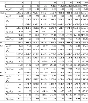
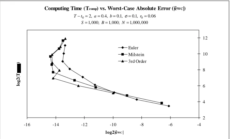
For the 2-year discount bond, Figures 1 and 2 show logarithmic (base 2) graphs of the absolute mean error and, more importantly, the absolute worst-case error against the size of the time-step. Although the different convergence orders of the used schemes are apparent for large values of the time-step (δ ≥2−2), the Milstein and third-order schemes quickly reach an error level of around |e$wc|≈2− =0 61.

14 _{basis points (bp) beyond which increasing}

Absolute Mean Error (|ê|) as a Function of Time-Step (δ)

-21 -19 -17 -15 -13 -11 -9 -7 -5

-7 -6 -5 -4 -3 -2 -1 0 1

log2(δ)

log2|

ê|

Euler Milstein 3rd Order

T− =t₀ 2,a=0 4. ,b=0 1. ,σ=0 1. ,r₀=0 06.

S=1 000, ;B=1 000, ;N=1 000 000, ,

Figure 1

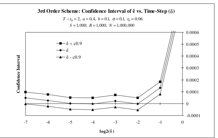
Worst-Case Absolute Error (|êWC|) as a Function of Time-Step (δ)

-15 -14 -13 -12 -11 -10 -9 -8 -7 -6 -5

-7 -6 -5 -4 -3 -2 -1 0 1

log2(δ)

log2|

ê

|

Euler Milstein 3rd Order

T− =t0 2,a=0 4. ,b=0 1. ,σ=0 1. ,r0=0 06.

S=1 000, ;B=1 000, ;N=1 000 000, ,

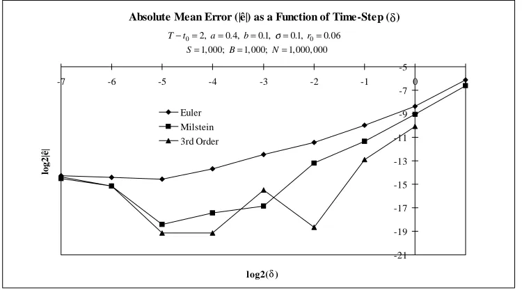
3rd Order Scheme: Confidence Interval of ê vs. Time-Step (δ)

-0.0001 0 0.0001 0.0002 0.0003 0.0004 0.0005 0.0006

-7 -6 -5 -4 -3 -2 -1 0

log2(δ)

Co

nfi

d

ence I

n

terv

a

l

ê + c0.9 ê ê - c0.9

T− =t0 2,a=0 4. ,b=0 1. ,σ=0 1. ,r0=0 06. S=1 000, ;B=1 000, ; N=1 000 000, ,

Figure 3

Worst-Case Absolute Error (|êWC|) as a Function of Time-Step (δ)

-12 -11 -10 -9 -8 -7 -6 -5

-7 -6 -5 -4 -3 -2 -1 0 1

log2(δ)

log2|ê

|

Euler Milstein 3rd Order

T− =t0 2,a=0 4. ,b=0 1. ,σ=0 1. ,r0=0 06. S=100; B=100; N=10 000,

Figure 4

Computing Time (Tcomp) vs. Worst-Case Absolute Error (|êWC|)

2 4 6 8 10 12

-16 -14 -12 -10 -8 -6 -4

log2|êWC|

log2(T

)

Euler Milstein 3rd Order

T− =t0 2,a=0 4. ,b=0 1. ,σ=0 1. ,r0=0 06.

S=1 000, ;B=1 000, ;N=1 000 000, ,

Figure 5

4. Variance Reduction Methods

4.1 Traditional Variance Reduction Methods

It is evident from the results so far, that for high-order discretization schemes to be of any practical use, we need methods to reduce the variance of the bond price estimator (18). Initially, we will focus on two widely used techniques from the classical Monte Carlo theory, namely antithetic variates and control variates. To briefly introduce these methods, let us restate the bond pricing problem in a slightly modified form. From (18), we know that discount bond prices can be approximated from the random variables

$ _{(~ , ~ ,..., ~ ) , ,2,...,}

IK f z z z j N

j j j

K j

where ~ , ~ ,..., ~zj zj zK j

1 2 is an independent sequence of standard Gaussian variables and

f:ℜ → ℜK is an (implicit) well-behaved function given by the discretization scheme used. Instead of using (28) directly to evaluate (18), the antithetic variate method uses the

N variables

$ _{, (~ , ~ ,..., ~ ) ( ~ , ~ ,..., ~ )} $ $ _{, ,2,...,}

IK A f z z z f z z z I I j N

j j j

K

j j j

K j K j K j

=1 + − − − = + − =

2

1

2 1

1 2 1 2

4

9 4

9

(29)

where the "mirror" process I$K− is obtained by changing the sign on all draws from the

standard Gaussian distribution. The mean of I$K A_, is clearly identical to that of I$K,

whereas the variance is

Vt I V I I I

Q

K A t Q

K K K

0 0

1

2 1

[$ , ]= [$ ] (

4

9

where ρ(I$K,I$K−) denotes the correlation coefficient between I$K and I$K−. If this

correlation coefficient is close to -1, the variance of I$K A_, will be significantly smaller

14 than the variance of I$K.

Whereas the antithetic variate method relies upon the existence of a process negatively correlated to I$K, the control variate method is based upon sampling a process positively

correlated to I$K. One way

15 _{to introduce a control variate is to consider an alternative short} rate model, say

d r I

r t

r I dt

r t

dW t t r r const D I

t t

r t t t

r t

t t t t

* * * * * * * * * * * ( , ) ( , ) , , . ,

0 0 0 0 0 1

for which an analytical solution to discount bond prices is known (like the CIR model (4) or the Vasicek model (5)). Now instead of (18), we write

$ _{( , )} $ $* *_{( , ) (}$ $* ₎ *_{( , )}

P t T

N I N I P t T N I I P t T

C K j j N K j j N K j K j j N 0 1 1 0 1 0

1 1 1

= − + = − +

= = =

∑

∑

∑

(32)

where P t T*( , )0 is the known theoretical value of the control variate bond price. The mean

and variance of P t T$C( , )0 are given by

E_tQ₀[P t T$C( , )]0 P t T( , )0 esys esys

*

= + − (33a)

V P t T

N V I V I COV I I

V e V e

NCOV I I

t Q C t Q K t Q K t Q K K t Q stat t Q stat t Q K K

0 0 0 0

0 0 0

0 1 2 2 [$ ( , )] [$ ] [$ ] ($ ,$ ) [$ ] [$ ] ($ ,$ ) * * * * = + − = + −

4

9

It follows easily from the triangle inequality that

|esys| C , |e* | C* |e e* | |e | |e* | (C C*)

n sys

n

sys sys sys sys

n

≤ δ ≤ δ ⇒ − ≤ + ≤ + δ (34)

From (33a) we can therefore conclude that if both (12) and (31) are discretized by nth-order weak schemes, the estimate P t T$C( , )0 will converge with (at least) weak order n as well.

Further, from (33b) we see that the variance of P t T$C( , )0 will be less than the variance of

estimate P t T$( , )0 (see (22)) if

COV I I V I I I V I

V I

t Q

K K t

Q

K K K

t Q K t Q K 0 0 0 0 1 2 1 2 ($ ,$ ) ($ ) ($ ,$ ) ( $ ₎ ($ ) * * * *

To ensure that (35) holds, it is important that the parameters of the control variate process (31) are chosen to match the dynamics of the original process (12) as closely as possible.

4.2 Application of Traditional Variance Reduction to the CIR Model

Whereas implementation of the antithetic variate method on the CIR model is straightforward, implementation of the control variate technique involves selecting an appropriate alternative process (31). Here, we will use the Vasicek process (5) which is structurally quite similar to the CIR process (4); Appendix B contains the Euler and Milstein discretization schemes for the Vasicek model. The third-order Vasicek scheme can be generated from (24). There are several ways to pick the parameters α , β, and κ in (5); we will choose the parameters to match the first and second moments of the CIR model16. From (6) and (7) we thus get

α=a, β=b, κ

σ

2

2 2 2

2

2 1

1

0

0 0 0

0

=

−

− − − − − −

− −

r e e b e

e

t

a T t a T t a T t a T t

( ) ( ) ( )

( )

4

9 4

9

4

9

(36)

PCIR - PVasicek for Different Bond Maturities

0 0.001 0.002 0.003 0.004 0.005 0.006 0.007 0.008

0 1 2 3 4 5 6 7 8 9 10

Maturity (T-t)

P

ri

ce D

ifference ($

)

High Volatility (a = 0.2, sigma = 0.125) Medium Volatility (a = 0.1, sigma = 0.075) Medium Volatility (a = 0.4, sigma = 0.1) Low Volatility (a = 0.6, sigma = 0.075)

b = 0.1, r0 = 0.06

Figure 6

Simulation Results for CIR Model

5-Year Discount Bond, Theoretical Value = 0.6642841

N=10 000, ;S=100;B=100

a=0 4. ,b=0 1. ,σ=0 1. ,r₀=0 06.

K 4 8 16 32 64 128 256

δ 1.25 0.625 0.3125 0.1563 0.07813 0.03906 0.01953

Crude Monte Carlo

Euler $/

VB

1 2 _{0.00579 0.00541 0.00557 0.00510 0.00576 0.00610 0.00686}

c0 9. 9.61E-4 8.98E-4 9.25E-4 8.46E-4 9.57E-4 1.01E-3 1.14E-3

Tcomp 0.34 0.68 1.35 2.75 5.34 10.78 21.3

Milstein $/

VB

1 2 _{0.00543 0.00519 0.00540 0.00506 0.00577 0.00611 0.00687}

c0 9. 9.01E-4 8.62E-4 8.97E-4 8.40E-4 9.57E-4 1.01E-3 1.14E-3

Tcomp 0.55 1.03 2.05 4.02 8.23 16.28 32.65

3rd Order $/

VB

1 2 _{0.00632 0.00590 0.00633 0.00577 0.00665 0.00718 0.00789}

c0 9. 1.05E-3 9.80E-4 1.05E-3 9.57E-4 1.10E-3 1.19E-3 1.31E-3

Tcomp 0.64 1.23 2.43 4.79 9.53 18.99 38.44

Antithetic Variate

Euler $/

VB

1 2 _{7.26E-4 7.30E-4 6.98E-4 6.33E-4 6.57E-4 6.10E-4 5.79E-4}

c0 9. 1.21E-4 1.21E-4 1.16E-4 1.05E-4 1.09E-4 1.01E-4 9.61E-5

Tcomp 0.52 0.97 1.89 3.71 7.49 15.21 30.14

Milstein $/

VB

1 2 _{5.52E-4 5.90E-4 5.48E-4 6.02E-4 6.57E-4 6.11E-4 5.83E-4}

c0 9. 9.17E-5 9.79E-5 9.09E-5 1.00E-4 1.09E-4 1.01E-4 9.68E-5

Tcomp 0.85 1.68 3.34 6.60 12.90 25.91 51.87

3rd Order $/

VB

1 2 _{7.08E-4 6.74E-4 6.41E-4 7.50E-4 7.96E-4 7.31E-4 6.96E-4}

c0 9. 1.18E-4 1.12E-4 1.06E-4 1.24E-4 1.32E-4 1.21E-4 1.16E-4

Tcomp 1.07 2.05 4.00 8.18 15.68 31.82 63.64

K 4 8 16 32 64 128 256

δ 1.25 0.625 0.3125 0.1563 0.07813 0.03906 0.01953

Control Variate

Euler $/

VB

1 2 _{0.00160 0.00136 0.00130 0.00124 0.00141 0.00153 0.00138}

c0 9. 2.65E-4 2.25E-4 2.16E-4 2.06E-4 2.35E-4 2.54E-4 2.30E-4

Tcomp 0.42 0.78 1.54 3.10 5.83 11.76 23.80

Milstein $/

VB

1 2 _{0.00130 0.00126 0.00120 0.00123 0.00141 0.00151 0.00137}

c0 9. 2.15E-4 2.08E-4 2.00E-4 2.05E-4 2.34E-4 2.51E-4 2.28E-4

Tcomp 0.65 1.24 2.37 4.64 9.11 18.03 36.21

3rd Order $/

VB

1 2 _{0.00165 0.00144 0.00142 0.00152 0.00164 0.00175 0.00160}

c0 9. 2.73E-4 2.40E-4 2.36E-4 2.53E-4 2.72E-4 2.90E-4 2.65E-4

Tcomp 0.71 1.39 2.86 5.43 10.92 21.8 42.30

Antithetic + Control Variate

Euler $/

VB

1 2 _{0.00111 0.00112 0.00110 0.00105 0.00113 0.00114 0.00097}

c0 9. 1.84E-4 1.86E-4 1.83E-4 1.74E-4 1.87E-4 1.90E-4 1.62E-4

Tcomp 0.59 1.22 2.31 4.49 7.87 16.99 32.91

Milstein $/

VB

1 2 _{0.00104 0.00103 0.00099 0.00104 0.00114 0.00114 0.00098}

c0 9. 1.73E-4 1.71E-4 1.64E-4 1.73E-4 1.89E-4 1.90E-4 1.63E-4

Tcomp 0.99 1.93 3.59 7.01 13.98 28.61 54.88

3rd Order $/

VB

1 2 _{0.00131 0.00119 0.00118 0.00131 0.00135 0.00136 0.00119}

c0 9. 2.17E-4 1.97E-4 1.96E-4 2.18E-4 2.24E-4 2.25E-4 1.97E-4

Tcomp 1.29 2.49 4.63 8.99 17.81 35.72 71.03

To aggregate the results in Table 2 and to properly account for the differences in computation time, we define an average efficiency ratio

E const

VB V V T T T

Euler B

Milstein B

rd comp

Euler comp

Milstein comp

rd

=

+ + + +

.

$ $ $3 3

4

94

9

where we pick the constant in the numerator to normalize E to 1 for crude Monte Carlo simulation. The results of this calculation are shown in Table 3 and graphed in Figure 7.

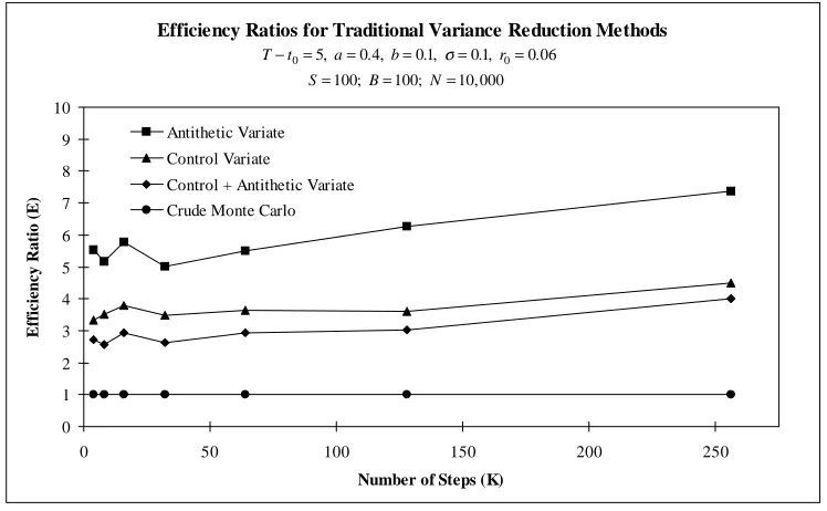
Efficiency Ratios for Simulation of 5-Year Discount Bond in CIR Model

N=10,000;S=100;B=100

a=0 4. ,b=01. ,σ=01. ,r0=0 06.

K 4 8 16 32 64 128 256

δ 1.25 0.625 0.3125 0.1563 0.07813 0.03906 0.01953

Crude Monte Carlo 1.00 1.00 1.00 1.00 1.00 1.00 1.00

Antithetic Variate 5.54 5.18 5.79 5.01 5.52 6.27 7.38

Control Variate 3.32 3.51 3.80 3.49 3.64 3.61 4.48

Antithetic + Control Variate

2.71 2.58 2.93 2.64 2.93 3.01 4.00

Efficiency Ratios for Traditional Variance Reduction Methods

0 1 2 3 4 5 6 7 8 9 10

0 50 100 150 200 250

Number of Steps (K)

Effi

ci

ency

R

a

ti

o

(E)

Antithetic Variate Control Variate

Control + Antithetic Variate Crude Monte Carlo

T− =t0 5,a=0 4. ,b=0 1. ,σ=0 1. ,r0=0 06.

S=100;B=100;N=10 000,

Figure 7

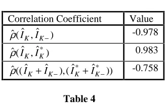
Sample Correlation Coefficients for CIR Model Euler Simulation of 5-Year Discount Bond

N=10,000;S=100;B=100; K=32

a=0 4. ,b=01. ,σ=01. ,r0=0 06.

Table 4

The correlation coefficients for both the antithetic and the control variate methods are very close to their optimal values of -1 and +1, respectively. Interestingly, however, the correlation between the combined variates (I$K+I$K−) /2 and ($ $ ) /

* *

IK+IK− 2 is negative.

According to (35), adding the control variate method to the antithetic method will thus cause an increase in variance, consistent with the experimental results in Table 2. Although there are other applications (see for example Clewlow and Carverhill (1994)) where the combination of the antithetic and control variate methods will outperform either method alone, it is obvious from the above findings that an uncritical combination of variance reduction techniques can lead to suboptimal results.

For completeness, Appendix C lists efficiency ratios for 1-, 2-, and 10-year discount bonds. Except for the 1-year bond where the control variate method slightly outperforms the antithetic variate method, the efficiency results are very similar to those of the 5-year bond. Notice, that the efficiency of the control variate method falls with increasing bond maturities, an effect that can easily be understood from Figure 6: the higher the bond maturity, the poorer the quality of the Vasicek control variate.

Correlation Coefficient Value

$($ ,$ )

ρ IK IK− -0.978

$($ ,$*)

ρ IK IK 0.983

$(($ $ ),($* $* ))

4.3 The Measure Transform Method

In the previous sections, we illustrated how knowledge about a simpler control variate process can, in principle, be used to improve simulation results. For the specific example of using the Vasicek model as a control variate process for the CIR model the results, however, were somewhat disappointing. In this section we will discuss an alternative, SDE-based method to incorporate results obtained from simpler processes into the simulation procedure. The method was proposed by Milstein (1988) and is based on a (reverse) application of the Girsanov Theorem for shift of probability measure (Karatzas and Shreve (1991), p. 190-201).

To introduce this technique, we consider a process θ_t and an equivalent probability measure Z under which

dWt dWt tdt

~

= +θ (38)

is a standard Brownian motion on ( , , )Ω F Z . Under technical conditions on θ_t (see footnote 6), the Girsanov Theorem asserts that the measure Z is related to Q through the Radon-Nikodym derivative

dQ

dZ = t sdWs− t sds

I

I

exp θ ~ θ

τ

τ ₁

2

2 0 0

(39)

where as before [ , ]t0 τ represents our bounded trading horizon. Corresponding to (39), we

introduce the likelihood ratio process

ξt t θ θ

Z

s s s

t t t

t

E dQ

dZ dW ds

= =exp

I

I

2

dξt =θ ξt tdWt ξt =

~ ,

0 1 (40)

which obviously is a martingale under Z. Expectations under Z and Q can now be shown to be related through

E_tQ X_t E_tZ X_{t t}

0[ ]= 0[ ξ ] (41)

for any absolutely integrable ℑ_t-measurable random variable Xt, t∈[ , ]t0 τ . Notice that

(41) is independent of the actual choice of ξ_t; if we can chose ξ_t such that the variance of the product Xtξt (under Z) is smaller than the variance of Xt (under Q), (41) can be used

as a variance reduction scheme.

We now return to the joint process (12) which we amend to include the likelihood ratio process (40). Under Z, we have

d r I

r t r t

r I dt

r t

dW r const D I

t t t

r t t r t t t

r t

t t

t t t t

ξ

µ θ σ σ

θ ξ ξ

0 _{0 0 0} 1

(42)

and the corresponding bond pricing equation

P t T Et I

Z T T

( , )0 = [ ξ ] (43)

The question now arises: how do we pick θt to minimize the variance of ITξT? If we

introduce the function17 hT:D×[ , ]t T0 → ℜ+ such that P t T( , )=h r tT( , )t , Appendix D

θ ∂ ∂

σ

t T t r t

T t

T t T

h r t r

r t

h r t g r t g D t T

= − ( , ) ( , )= × → ℜ

( , ) ( , ) , : [ , ]0 (44)

will reduce the variance of ITξT to zero (under Z). Unfortunately, we generally do not

know the explicit relation P t T( , )=h r tT( , )t -- if we did, there would be no need to evaluate

(43) through simulation. However, in many circumstances we can come up with a good guess for (44), for example by using known bond formulas for simpler interest rate models. Suppose, say, we believe that our interest rate model yields bond prices which are reasonably close to those of the Vasicek (5) model (with appropriately chosen parameters). Applying the Vasicek bond formula (11) to (44) yields the simple result

g_TVasicek r t_t D t T _r r t_t D t T e

T t

( , ) ( , ) ( , ), ( , )

( )

= σ = − − −

α

α

1

(45)

Discretization schemes for the SDE (42) can be derived along the same lines as in Section 3.1. The Euler and Milstein schemes for rt and It will be identical to (16a-b) and (17a-b)

provided µ_r( , )r t_t is replaced by µ_{r MT,} ( , )r t_t =µ_r( , )r t_t −g_T( , )r t_t σ_r( , )r t_t . The schemes for the likelihood ratio process ξ_t are as follows

Euler:

$ $ _{( ($, )~ ) , , ,..., , $ ,} $

Milstein: $ $ ($, ) ($, ) ($, )~ ($, ) ($, ) ($, ) ~ ($, ) ($, ) ~ , , ,..., , $ ξ

ξ δ δ δ δ δ

δ δ δ δ δ

δ δ δ

i i

T i T i T i i

MT T i T i T i i

T i T i i

L g r t i g r t i g r t i z

L g r t i g r t i L g r t i z

L g r t i g r t i z i K

+ + + + = − + + + + + + + + + + + + + + = − 1 1 0 0 2 0 1 0 0 0 1 0 1 1 0 0 2 1 2 1 1 2 1 2 1

2 0 1 1

4

9

4

9

4

9

(47)

where the differential operator LMT

0

is identical to L0 in (15), except that µ_r( , )r t_t must be replaced by µ_{r MT,} ( , )r t_t =µ_r( , )r t_t −g_T( , )r t_t σ_r( , )r t_t .

4.4 Application of the Measure Transform Method to the CIR Model

We now turn to applying the measure transform method to the CIR process (4). We will use the Vasicek model (with α =a , see (36)) to generate the function h r tT( , )t ; consequently,

the volatility of the likelihood ratio process is given by (45). From (10), we note that the (continuous-time) perfect choice of gT( , )r tt is

g r t B t T r B t T e

a a e a

T CIR

t t

a T t a T t

( , ) ( , ) , ( , ) ( ) ( )( ) ( ) ( ) = = − + + − + + + − + − σ σ σ σ σ 2 1

2 1 2 2

2 2

2 2 2

2 2 2 2 2

(48)

B(t,T) and D(t,T) for Different Bond Maturities

0.5 1 1.5 2 2.5 3 3.5 4 4.5 5

0 1 2 3 4 5 6 7 8 9 10

Maturity (T-t)

B(t,T) , D

(t,T)

B(t,T) (a = 0.1, sigma = 0.075) D(t,T) (a = 0.1, sigma = 0.075) B(t,T) (a = 0.4, sigma = 0.1) D(t,T) (a = 0.4, sigma = 0.1) B(t,T) (a = 0.6, sigma = 0.075) D(t,T) (a = 0.6, sigma = 0.075)

b = 0.1, r0 = 0.06

Figure 8

Applying (16a-b), (17a-b), (46), and (47) to the CIR process now yields the following schemes

Euler Scheme:

$ $_{( $ ) ,}

Ii+1=Ii1−riδ (48a)

$ $ _{( ( , ) |$|~ ) ,}

ξi+1=ξi1+D t0+iδ T σ r zi i+1 δ (48b)

$ $ $( ( , ))

|$|~ , , ,..., , $ , $ $

r r ab r a D t i T

r z i K r r I

i i i

i i t

+

+

= + − + + +

= − = = =

1

2 0

1 0 1 1 0 0 0 0 1

σ δ δ

σ δ ξ

4

9

Milstein Scheme:

$ $ ( ) ( , )$ ( , ) |$|~ ( , ) |$| ( , ) |$| ~ ( ) ( , )$ ~ , ξ ξ

ψ _{δ δ δ σ δ}

δ σ

δ

σ _{δ δ}

ψ _{δ δ}

i i

i

i i i

i i i i i i a

D t i T r D t i T r z

D t i T

r a

D t i T r ab z

a

D t i T r z

+ + + + = − −

0 0 1

0 0 2 1 0 1 2 1 2 1 2 4 2 1 4 2 1 2 (49b) $ $ $ |$|~ |$| |$| ~ $ ( , ) ~ _{, , ,..., , $ , $}

r r ab r r z

r ab r z

r a D t i T ba

z i K r r I

i i i i i i

i

i i i

i i i

i t + + + + = +

2 4 2

2 1 2 0 0 4 4 1 4 3 1 2

4 0 1 1 0 1

ψ σ δ σ δ σ σ ψ δ δ

ψ σ δ σ ψ δ

σ _δ

4

9

4

9

(49c)

where

ψi≡ +a D t(0+iδ, )T σ

2

We notice that, similar to the control variate technique, the measure transformation method can be combined with the antithetic method. As the measure transformation method is not based upon a correlation argument, we are less likely to experience the difficulties we encountered in Section 4.2 when we attempted to combine antithetic and control variates.

Simulation Results for CIR Model

5-Year Discount Bond, Theoretical Value = 0.6642841

N=10,000;S=100;B=100

a=0 4. ,b=01. ,σ=01. ,r0=0 06.

K 4 8 16 32 64 128 256

δ 1.25 0.625 0.3125 0.1563 0.07813 0.03906 0.01953

Measure Transformation

Euler $/

VB

1 2 _{2.21E-3 1.08E-3 5.05E-4 2.67E-4 1.51E-4 8.80E-5 7.53E-5}

c0 9. 3.68E-4 1.79E-4 8.38E-5 4.43E-5 2.51E-5 1.46E-5 1.25E-5

Tcomp 0.44 0.87 1.70 3.44 6.83 13.58 26.80

Milstein $/

VB

1 2 _{5.30E-4 1.84E-4 9.00E-5 6.04E-5 5.82E-5 6.75E-5 7.25E-5}

c0 9. 8.80E-5 3.06E-5 1.49E-5 1.00E-5 9.66E-6 1.12E-5 1.20E-5

Tcomp 0.69 1.36 2.66 5.43 10.76 21.48 42.75

3rd Order $/

VB

1 2 _{1.08E-3 4.96E-4 2.50E-4 1.49E-4 9.20E-5 8.46E-5 8.68E-5}

c0 9. 1.79E-4 8.23E-5 4.15E-5 2.48E-5 1.53E-5 1.40E-5 1.44E-5

Tcomp 0.88 1.70 3.37 6.83 13.25 26.40 53.03

Measure Transformation + Antithetic Variate

Euler $/

VB

1 2 _{7.11E-4 3.02E-4 1.64E-4 8.71E-5 6.74E-5 4.97E-5 3.24E-5}

c0 9. 1.18E-4 5.02E-5 2.72E-5 1.45E-5 1.12E-5 8.25E-6 5.37E-6

Tcomp 0.69 1.34 2.62 5.11 10.22 20.45 40.93

Milstein $/

VB

1 2 _{4.69E-4 1.67E-4 5.72E-5 2.14E-5 1.18E-5 9.51E-6 8.46E-6}

c0 9. 7.79E-5 2.77E-5 9.49E-6 3.56E-6 1.96E-6 1.58E-6 1.41E-6

Tcomp 1.20 2.25 4.45 8.91 17.79 35.56 70.81

3rd Order $/

VB

1 2 _{4.79E-4 1.99E-4 7.06E-5 2.98E-5 1.70E-5 1.29E-5 1.02E-5}

c0 9. 7.95E-5 3.31E-5 1.17E-5 4.95E-6 2.82E-6 2.15E-6 1.70E-6

Tcomp 1.48 2.92 5.78 11.45 22.80 45.49 90.69

Efficiency Ratios for Simulation of 5-Year Discount Bond in CIR Model

N=10,000;S=100;B=100

a=0 4. ,b=01. ,σ=01. ,r0=0 06.

K 4 8 16 32 64 128 256

δ 1.25 0.625 0.3125 0.1563 0.07813 0.03906 0.01953

Crude Monte Carlo 1.00 1.00 1.00 1.00 1.00 1.00 1.00

Antithetic Variate 5.54 5.18 5.79 5.01 5.52 6.27 7.38

Measure Transformation 3.49 7.02 15.45 24.58 45.17 60.53 69.48

Measure Transformation + Antithetic Variate

4.80 11.15 26.92 52.22 85.96 122.01 193.22

Table 6

The data in Table 6 is graphed in Figure 9. Except for very large time-steps (>1 year in our example), the combined method of measure transformation and antithetic variates is far superior to any of the traditional variance reduction methods tested in Section 4.2. Notice that the quality of the measure transformation method improves significantly as the number of time steps in each simulation path is increased. This behavior is not surprising given that the method has been designed around the continuous-time limit of the discretized processes. The tendency of the measure transform method to improve with increasing number of discretization steps is attractive since it complements the behavior of the systematic error in the SDE discretization scheme; increasing the number of discretization steps will improve

both esys and e$stat.

Efficiency Ratios for Measure Transformation Method

0 20 40 60 80 100 120 140 160 180 200

0 50 100 150 200 250

Number of Steps (K)

Effi

ci

ency

R

a

ti

o

(E)

Measure Transformation + Antithetic Variate Measure Transformation

Antithetic Variate

T− =t₀ 5,a=0 4. ,b=0 1. ,σ=0 1. ,r₀=0 06.

S=100;B=100;N=10 000,

Figure 9

4.5 Quasi-Random Sequences

As mentioned in the introduction, so-called quasi-random sequences have recently been applied quite successfully to certain classes of finance problems involving explicitly solvable SDEs. In this and the following section, we will investigate whether this promising technique is equally useful for the simulation of non-solvable SDEs.

To introduce the method of quasi-random sequences, consider writing equation (28) as

$ _{(~ , ~ ,..., ~ ) (~ , ~ ,..., ~ ), ,2,...,}

IK f z z z k u u u j N

j j j

K

j j j

K j

= 1 2 = 1 2 =1 (50)

where ~ , ~ ,..., ~uj uj uK j

1 2 is an independent sequence of standard uniform U(0,1)-variables and

distribution function or through the (inverse) Box-Mueller transformation. With (50), the expectation of I$K can now be written formally as an integral over the K-dimensional

hypercube

E_tQ I_K k x x x_K dx dx dx_K k x dx

K K

0[ _{0 1} 1 2 1 2 _{0 1}

$ ] ( , ,..., ) ( )

[ ; ] [ ; ]

=

I

I

Given some deterministic or random scheme to sample N K-tuples x xr r1, 2,...,xrN, we

consider estimating (51) through

E I

N k x

t Q

K j

j N

0

1

1

[$ ]≈ ( )

=

∑

(52)

which is identical to (18), except that we have not in (52) specified which sampling scheme is used. If the sampling scheme is Monte-Carlo simulation (i.e. based on pseudo-random number generators), we know that the expected error on (52) is independent of the dimension K and proportional to N−1 2/ . To improve the convergence properties of (52), several deterministic sampling algorithms have been suggested instead of Monte Carlo simulation. One class of such algorithms is based on the generation of quasi-random or low

discrepancy sequences, i.e. sequences which fill out the hypercube in a cluster-free,

self-avoiding way18. Specific algorithms for generating quasi-random numbers have been suggested by Halton (1960), Sobol (1967), and Faure (1982), among others. For a very readable introduction to Halton and Sobol sequences, see Press et al (1992), chapter 7. Faure sequences are discussed in Bouleau and Lepingle (1994), chapter 2C, and Joy (1994).

k x dx

N k x Var k O N N

K j

j

N K

( ) ( ) ( ) (ln )

[ ; ]

r r r

0 1

1

1

I

∑

=

(53)

where Var(k) is the (bounded) variation of k on [ ; ]0 1K in the sense of Hardy and Krause

(Niederreiter (1992), p. 19). Although the O

4

9

O N( −1 2/ ) as N→ ∞, it is not small for realistic N for problems of large dimension K:

Convergence Orders for Quasi-Random Sequences and Crude Monte Carlo

N=10,000 N=1,000,000

K Quasi-Random Monte Carlo Quasi-Random Monte Carlo

1 9.21E-4 1.00E-2 1.38E-5 1.00E-3

5 6.63E+0 1.00E-2 5.03E-1 1.00E-3

10 4.39E+5 1.00E-2 2.53E+5 1.00E-3

50 1.64E+44 1.00E-2 1.04E+51 1.00E-3

Table 7

In practice, however, the upper bound provided by the Koksma-Hlawka inequality often turns out to significantly understate the true convergence speed of quasi-random sequences; in Brotherton-Ratcliffe (1994b), for example, Sobol sequences outperform crude Monte Carlo for option pricing applications with K=48 dimensions. For problems involving numerical solution of SDEs, it is nevertheless worrying that the performance of quasi-random sequences decreases when the dimension goes up. An attempt to improve the accuracy of the systematic error esys through an increase in the number of discretization

steps might thus be countered by decreased accuracy on the random error e$stat.

however, not recommended to combine Sobol sequences with antithetic variates, as the inclusion of "mirror paths" is likely to affect the discrepancy of the sequence adversely.

4.6 Application of Sobol Sequences to the CIR Model

As experimental results by Paskov (1994) and Brotherton-Ratcliffe (1994b) indicate that Sobol sequences frequently outperform both Halton and Faure sequences, this paper will only discuss the application of Sobol sequences. For the practical generation of Sobol points, we have relied upon the highly efficient algorithm by Antonov and Saleev (1979) which is described in detail in Press et al (1992). The generation of the primitive polynomials needed in the Anotonov and Saleev’s algorithm has been based on Knuth (1981), chapter 3.

Again using the example of a 5-year bond with N=10,000 (results for other bonds are listed in Appendix C), we get the results shown in Tables 8 and 9. As a reflection of the deterministic nature of Sobol sequences, in Table 8 we have replaced standard deviation

$

VB with the root-mean-square error (relative to the sample mean) RMSB; both quantities

Simulation Results for CIR Model

5-Year Discount Bond, Theoretical Value = 0.6642841

N=10,000;S=100;B=100

a=0 4. ,b=01. ,σ=01. ,r0=0 06.

K 4 8 16 32 64 128 256

δ 1.25 0.625 0.3125 0.1563 0.07813 0.03906 0.01953

Sobol Sequence

Euler RMSB 1.42E-3 1.78E-3 1.85E-3 2.44E-3 3.55E-3 3.86E-3 3.87E-3

Tcomp 0.34 0.59 1.14 2.2 4.32 8.32 16.76

Milstein RMSB 1.28E-3 1.61E-3 1.81E-3 2.41E-3 3.53E-3 3.82E-3 3.87E-3

Tcomp 0.50 0.96 1.80 3.54 7.01 13.94 27.88

3rd Order RMSB 1.41E-3 1.78E-3 2.08E-3 2.88E-3 4.17E-3 4.39E-3 4.17E-3

Tcomp 0.63 1.13 2.19 4.27 8.47 16.81 33.09

Sobol Sequence + Control Variate

Euler RMSB 6.76E-4 1.07E-3 1.20E-3 1.41E-3 1.31E-3 1.43E-3 1.67E-3

Tcomp 0.43 0.71 1.21 2.43 4.78 9.49 18.66

Milstein RMSB 5.78E-4 8.98E-4 1.08E-3 1.31E-3 1.25E-3 1.40E-3 1.65E-3

Tcomp 0.62 1.12 2.04 3.75 7.45 14.49 28.91

3rd Order RMSB 7.55E-4 9.65E-4 1.21E-3 1.52E-3 1.50E-3 1.70E-3 2.03E-3

Tcomp 0.69 1.24 2.54 4.63 9.36 18.47 37.08

Sobol Sequence + Measure Transformation

Euler RMSB 6.87E-4 3.03E-4 2.83E-4 1.92E-4 1.10E-4 5.03E-5 4.31E-5

Tcomp 0.46 0.82 1.56 2.98 5.80 11.62 22.36

Milstein RMSB 2.46E-4 8.55E-5 2.84E-5 2.19E-5 2.75E-5 3.62E-5 3.83E-5

Tcomp 0.66 1.31 2.44 4.68 9.30 18.88 36.44

3rd Order RMSB 3.27E-4 1.81E-4 9.73E-5 8.67E-5 6.42E-5 4.78E-5 4.74E-5

Efficiency Ratios for Simulation of 5-Year Discount Bond in CIR Model

N=10,000;S=100;B=100

a=0 4. ,b=01. ,σ=01. ,r0=0 06.

K 4 8 16 32 64 128 256

δ 1.25 0.625 0.3125 0.1563 0.07813 0.03906 0.01953

Crude Monte Carlo 1.00 1.00 1.00 1.00 1.00 1.00 1.00

Antithetic Variate 5.54 5.18 5.79 5.01 5.52 6.27 7.38

Sobol Sequence 4.44 3.50 3.42 2.38 1.89 1.89 2.16

Sobol Sequence + Control Variate

7.68 5.39 4.99 4.02 4.78 4.64 4.42

Sobol Sequence + Measure Transformation

10.81 22.57 33.68 44.93 77.23 120.81 147.07

Antitethetic Variate + Measure Transformation

4.80 11.15 26.92 52.22 85.96 122.01 193.22

Note: The highest efficiency ratio for each step-size has been highlighted

Table 9