FORMOSAT/COSMIC observations
Amelia Naomi Onohara1, Inez Staciarini Batista2, and Paulo Prado Batista2
1Brazilian Space Agency, SPO Sul, Area 5, Quadra 3, Bloco A, 70610-200, Brasilia, DF, Brazil 2National Institute for Space Research, Av dos Astronautas, 1758, Jd da Granja, 12227-010, Sao Jose dos Campos, SP, Brazil
Correspondence:Amelia Naomi Onohara (amelia.onohara@aeb.gov.br)
Received: 24 August 2017 – Revised: 6 February 2018 – Accepted: 13 February 2018 – Published: 21 March 2018
Abstract.The main purpose of this study is to investigate the four-peak structure observed in the low-latitude equatorial ionosphere by the FORMOSAT/COSMIC satellites. Longi-tudinal distributions of NmF2 (the density of the F layer peak) andhmF2 (ionospheric F2-layer peak height) averages, obtained around September equinox periods from 2007 to 2015, were submitted to a bi-spectral Fourier analysis in or-der to obtain the amplitudes and phases of the main waves. The four-peak structure in the equatorial and low-latitude ionosphere was present in both low and high solar activity periods. This kind of structure possibly has tropospheric ori-gins related to the tidal waves propagating from below that modulate the E-region dynamo, mainly the eastward non-migrating diurnal tide with wavenumber 3 (DE3, “E” for eastward). This wave when combined with the migrating di-urnal tide (DW1, “W” for westward) presents a wavenumber-4 (wave-wavenumber-4) structure under a synoptic view. Electron densi-ties observed during 2008 and 2013 September equinoxes revealed that the wave-4 structures became more prominent around or above the F-region altitude peak (∼300–350 km). The four-peak structure remains up to higher ionosphere alti-tudes (∼800 km). Spectral analysis showed DE3 and SPW4 (stationary planetary wave with wavenumber 4) signatures at these altitudes. We found that a combination of DE3 and SPW4 with migrating tides is able to reproduce the wave-4 pattern in most of the ionospheric parameters. For the first time a study using wave variations in ionospheric observa-tions for different altitude intervals and solar cycle was done. The conclusion is that the wave-4 structure observed at high altitudes in ionosphere is related to effects of the E-region dynamo combined with transport effects in the F region.
Keywords. Ionosphere (equatorial ionosphere)
1 Introduction
The equatorial ionization anomaly (EIA) is an important characteristic of the low-latitude and equatorial ionosphere. The EIA is produced by the equatorial plasma fountain ef-fect that elevates the equatorial and low-latitude ionospheric plasma to higher altitudes in the F region. The fountain ef-fect is a daytime phenomenon characterized by the upward plasma drift that results from interactions between electric and magnetic fields in the E region. In the F region, the trans-port processes are imtrans-portant because of the small recombina-tion rates. Due to the acrecombina-tion of gravity and the pressure gradi-ent, this plasma diffuses down along the magnetic field lines to latitudes away from the geomagnetic equator (15–20◦), creating two crests with larger ionospheric plasma density in both hemispheres north and south of the magnetic equator (Namba and Maeda, 1939; Appleton, 1946; Rishbeth, 2000; Abdu, 2005).
460 A. N. Onohara et al.: Wavenumber-4 structures observed in the low-latitude ionosphere
structures seen in the ionosphere are related to the DE3 wave (the eastward non-migrating diurnal tide with wavenumber 3, “E” for eastward) that comes from latent heating in the tro-posphere. The wave-4 structure is a result of the predom-inant wave-4 topography, which is reflected in the diurnal and semidiurnal components of the latent heating rates due to deep tropical convection (Forbes, 2007).
The four peaks in the longitudinal structure in the equato-rial anomaly were first observed by Sagawa et al. (2005) us-ing atomic oxygen OI 135.6 nm nightglow emission images obtained by far ultraviolet (UV) emission from IMAGE (Im-ager for Magnetopause-to-Aurora Global Exploration) satel-lite observations from March to June 2002. The authors sug-gested that the possible cause of these structures could be attributed to non-migrating tides propagating from below be-cause factors like those related to differences between the ge-omagnetic and the geographic equator or the declination an-gle of the geomagnetic lines could not explain the observed four-peaked structure.
The Sagawa et al. (2005) supposition was confirmed by Immel et al. (2006) who indicated the existence of good cor-relation between the Sagawa et al. (2005) ionospheric imag-ing results and the upper atmosphere tidal parameters from the GSWM (Global Scale Wave Model). According to the authors, the tidal amplitudes decay in the E-region altitudes, making it impossible to affect the F region directly. In this way, a possible scenario would be one in which the tidal modulations could reach higher ionospheric altitudes by the E-layer dynamo mechanism.
Hagan et al. (2007) reported a series of simulations with the TIME-GCM (Thermosphere Ionosphere Mesosphere Electrodynamics general circulation model) which repro-duced the IMAGE observational results and confirmed that tides coming from the lower atmosphere could affect the EIA and consequently impact the ionosphere. The results identi-fied that the non-migrating tidal component responsible for the EIA four-peak structure is the DE3.
Non-migrating tides are global-scale waves with periods that have harmonics of a solar day and their origin is as-sociated with interactions between tides and gravity waves, gravitational pull of the Sun, large-scale latent heat release, absorption of solar radiation, nonlinear interactions between particular sets of global-scale waves and other interactions (Hagan and Forbes, 2003). The migrating tides move with the apparent motion of the Sun when they are observed from the ground, and their origin is associated with the absorption of infrared light in the troposphere and the UV light by ozone in the stratosphere.
The wave-4 structures can be noticed in periods of low and high solar activity. According to Scherliess et al. (2008), this is indicative of the fact that the coupling between the lower atmosphere and the ionosphere occurs independently of solar flux conditions. The authors used more than 5 mil-lion low-latitude TEC observations from the TOPEX (Ocean Topography Experiment) satellite, from August 1992 until
October 2005. They found that the longitudinal TEC struc-ture was not changed by the solar cycle conditions.
Oberheide et al. (2011a), using TIMED (Thermosphere Ionosphere Mesosphere Energetics and Dynamics) temper-ature and wind observations, from SABER (Sounding of the Atmosphere using Broadband Emission Radiometry) and TIDI (TIMED Doppler Interferometer) instruments, respec-tively, studied the contributions to the four-peak structure in the ionosphere of the following non-migrating tides: DW5, DE3, SW6, SE2, TW7 and TE1 (D, S and T for diurnal, semidiurnal and terdiurnal tides, respectively. W and E are for westward and eastward, respectively; the numbers are related to the tidal wavenumbers). All these waves can be observed as having a four-peak structure by the quasi-Sun-synchronous satellite using satellite sampling. Besides the tidal waves, the study also considered the stationary plane-tary wave with wavenumber 4 (SPW4). They demonstrated that the wave-4 structure in the E region was caused not only by the DE3 but also by a number of other waves, mainly the SE2 tidal component and SPW4. They also concluded that the modes TE1, DW5, SW6 and TW7 did not add substan-tially to the wave-4 amplitude.
Using the NCAR (National Center for Atmospheric Re-search) TIME-GCM model, Pedatella et al. (2012) per-formed numerical simulations using DE3, SE2 and SPW4 waves, for solar minimum conditions during the Septem-ber equinox, in order to study the formation of the four-peak structure in the low-latitude ionosphere. Their study presented results indicating that SE2 is not a contributor to the wave-4 longitude variation. The authors indicated that the SPW4 could be a result of a nonlinear interaction between DE3 and DW1 (the migrating diurnal tide, “W” for west-ward). It was also shown that the four-peak structure noticed in the September equinox was carried mainly by a combina-tion of DE3 and SPW4 waves.
Figure 1.Magnetic latitude interval of observations. Illustration of the ionospheric data used in the present study, which includes observations in the region±20◦around the magnetic equator. The example above is theNmF2 data taken during a time interval between 12:00 and 14:00 LT.
Waves’ amplitudes considered in their study also showed dif-ferences for both hemispheres.
The main subject of the present study is to observe the wave-4 structures in ionospheric parameters during different solar activity periods around the September equinox and ver-ify which waves will result using bi-spectral Fourier analysis fromNmF2 (the density of the F layer peak),hmF2 and Ne observations. It is know that large ionospheric variabilities in these parameters come from variation in the electric fields and winds, mainly due to ion–neutral coupling and electro-dynamic perturbations (Abdu, 2016). The hmF2 is related to effects of ionospheric dynamo, which consequently is re-sponsible for plasma uplift from low to high altitudes in the ionosphere. The fountain effect elevates ionospheric plasma in the regions near the magnetic equator to high altitudes, where it diffuses down through the geomagnetic field lines to latitudes located around 15–20◦from the magnetic equator. In this way it affects the electron density distribution. It will be possible to see which waves are more related to the wave-4 pattern, mainly when it appears more prominently. Studies in the literature have discussed that waves of tropospheric ori-gin could modify the ionosphere through the dynamo mech-anism or through direct upward propagation (Forbes, 1996). Some ionospheric perturbations can also be generated in situ.
2 Observations and results
The Formosa Satellite 3, also known as Constellation Ob-serving System for Meteorology, Ionosphere, and Climate (FORMOSAT-3/COSMIC or F3/C), is a set of six microsatel-lites that monitor atmosphere and space weather with instru-ments of radio occultation observations at altitudes ranging from the troposphere to the ionosphere (Lin et al., 2007c). The satellites have their final orbit at an altitude of 800 km
and a GPS receiver is used to obtain the atmospheric and ionospheric measurements through phase and Doppler shifts of radio signals. From the Ne profiles, theNmF2 andhmF2 can be calculated. The COSMIC satellites give around 24 h of LT coverage globally and ∼2200 electron density ver-tical profiles per day. The COSMIC observations provide global coverage of electron density profiles with uniform dis-tribution and good resolution. More details can be found in Pancheva and Mukhtarov (2010, 2012) and Ely et al. (2012). The COSMIC data are available for download from the website: http://cdaac-www.cosmic.ucar.edu/cdaac/products. html.
462 A. N. Onohara et al.: Wavenumber-4 structures observed in the low-latitude ionosphere
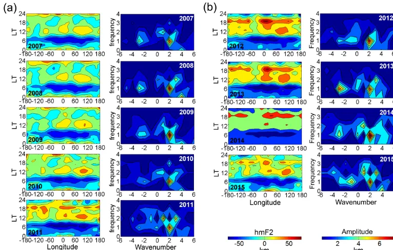
Figure 2.NmF2 LT contour plots.(a)LT×longitudeNmF2 contour plots from 2007 to 2015 around September equinoxes.(b)Amplitudes obtained for non-migrating tides indicating their frequency (1/day) and respective zonal wavenumber. The corresponding year for each plot is indicated in the graphs.
of data to set up the temporal and longitudinal averages for each parameter, as we can see in Fig. 1. After this process, the data were interpolated in order to obtain a 32×32 matrix. So, for each year,NmF2 andhmF2 intensity matrices from 0 to 24 h in time, and from−180 to 180◦in longitude, were ob-tained. Applying the two-dimensional fast Fourier transform (fft2) analysis over these matrices, phases and amplitudes of the waves present in these distributions were obtained.NmF2 andhmF2 variations were plotted in Figs. 2 and 4, respec-tively, with their corresponding amplitudes calculated from spectral analysis results.
Figure 2 shows the LT versus longitude maps averaged for NmF2 variations (left) and the frequencies (1/day) and zonal wavenumbers of the main non-migrating tides’ ampli-tudes obtained by two-dimensional Fourier spectral analysis, or fft2 analysis (right). The variations mean that zonal mean
NmF2 was subtracted from observations in order to obtain variations around zero. The fft2 is a MatLab routine and it computes Fourier coefficients in one dimension, in time for example, and then using the resulting coefficients, a new set of coefficients is computed in the other dimension, in this example, in space. In the continuous Fourier transform if a quantity with a unit A is computed in the frequency space, then the unit is A Hz−1. Since the fft2 routine used in this study is a discrete Fourier transform, the units are the same as the original data. These results encompass all the years used in this study. In the graphs on the left the maximum in-tensities of NmF2 are usually observed during the daytime
when the photoionization is higher. For higher solar periods,
NmF2 increases due to variations in the radiation intensity that cause changes in the electron–ion pairs’ production in the ionosphere. Visually the wave-4 patterns can be observed in 2008, 2009 and 2010. These four peaks are usually lo-cated in the Central Pacific (∼ −180 to −120◦ longitude), South America (∼ −120 to−60◦longitude), Africa (∼ −20 to 20◦ longitude) and Southeast Asia (∼80 to 120◦ longi-tude) (Lin et al., 2007c). From 2011 onward these structures are not well defined in comparison with those observed dur-ing the low solar activity years.
Figure 3.NmF2 relative amplitudes.NmF2 relative amplitudes calculated for periods around September equinoxes from 2007 to 2015 for some waves’ signatures observed in Fig. 2, mainly those related to the wave-4 structure, such as SE2, DE3 and SPW4, and those related to the offset between the geographic and geomagnetic coordinates, such as SPW1 and DW2. The F10.7 solar flux is plotted in the top graph, together with the DW1 relative amplitude.
thermospheric altitudes is caused by EUV (extreme ultravio-let radiation) forcing.
Observing the panels on the right in Fig. 2, it can be no-ticed that the DE3 wave is more pronounced during 2007, 2008 and 2015. In 2009 and 2010, the DE3 amplitude does not show a significant presence. In 2011 and 2012, DE3 ap-pears but with small amplitude in comparison with other waves. In 2013 and 2014, DE3 seems to be associated with other tidal modes, like SE1. SW1 is seen in all the years and is more pronounced during 2009, 2010 and 2012. This wave results from the coupling between SPW1 and SW2 (Jones et al., 2013). DW2 can be noticed in 2007, 2008, 2013, 2014 and 2015. Other waves like SPW1 and SPW4 can also be observed in some of these figures.
The wave-4 structures are usually related to DE3, SPW4 and SE2 non-migrating waves, which are of tropospheric origin. The fft2 analysis plots in the Fig. 2 do not indi-cate SE2 features. According to Jones et al. (2013), DW2 and D0 are generated in situ in the upper thermosphere due to the non-dipole nature of the geomagnetic field. These two non-migrating tides come from the interaction between SPW1 (related to the offset between the geomagnetic and ge-ographic poles) and DW1 (migrating diurnal tide). The off-set between the magnetic and geographic equator and differ-ences in magnetic declination are the cause for the longitude variation of the neutral winds in the equatorial region (Lei et al., 2007).
Figure 3 exhibits DE3, SPW4, SE2, SPW1, DW1 and DW2 relative amplitudes obtained from the results presented in Fig. 2. The relative amplitudes were calculated using the ratio between the amplitude of the selected wave and the maximum zonal mean because the absolute amplitudes re-flect the semiannual and solar cycle variations of the Ne zonal mean. The upper plot shows the diurnal migrating tide (DW1) relative amplitude and the F10.7 solar flux. We can see that the solar flux increased from 2007 to 2015, whereas the DW1 relative amplitude showed an opposite behavior. In
the bottom plot of Fig. 3, we can see some non-migrating and stationary waves’ relative amplitudes. DE3 and SPW4 show decreasing values as the solar flux increases. SE2 is a wave of tropospheric origin, also related to wave-4 structure, but in this example it does not show substantial variation. DW2, which appeared in several spectral plots in Fig. 2, also does not show great variation through the years, and the SPW1 wave has its maximum in 2011, when the high solar activity period starts.
Figure 4 shows longitudinal local-time-averaged distri-butions forhmF2 (left) with their respective non-migrating (right) tidal amplitudes. In the panels on the left it is possi-ble to see the wave-4 structures in practically all years, ex-cept 2010 and 2011. The F-layer elevation after 18:00 LT (highhmF2 values) for high solar activity periods is a sig-nature of the fountain effect intensification after the sunset because of the pre-reversal peak in the vertical drift (see, for example, Batista and Abdu, 2004). The right plots of Fig. 4 show that the DE3 wave is present practically in all the years, being more pronounced during 2007, 2008, 2009, 2013 and 2014. In other years its amplitude is smaller or not evident in the graphs. DW2 mode has significant amplitudes in all the years. The SPW4 wave is clearly visible from 2007 to 2010 and in 2015. The SW1 mode is present in the years 2007, 2011, 2014 and 2015. SW1 and SW3 are supposed to be pro-duced by the SPW1 and SW2 (semidiurnal migrating tide) coupling. SPW4 can also be noticed in the right figures.
464 A. N. Onohara et al.: Wavenumber-4 structures observed in the low-latitude ionosphere
[image:6.612.105.488.66.310.2]Figure 4. (a)LT×longitudehmF2 contour plots from 2007 to 2015 around September equinoxes.(b)Amplitudes obtained for non-migrating tides indicating their frequency (1/day) and respective zonal wavenumber. The corresponding year for each plot is indicated in the graphs.
Figure 5.hmF2 relative amplitudes for periods around September equinoxes from 2007 to 2015. The same waves amplitudes plotted in the Fig. 3 were considered here for the same reasons pointed earlier. F10.7 solar flux is plotted in the top graph with the DW1 relative amplitude. The results show different results showed in the Fig. 3.
different time constants to mechanical forcing, as discussed in Batista et al. (2011).
Electron densities (Ne) for 2 years with different levels of solar activity, 2008 and 2013, around the September equinox, were selected in order to see which wave signatures will ap-pear in these ionospheric parameters at different altitude in-tervals. Ne average matrices taken at each 50 km interval, from 100 to 800 km, were created. Each Ne matrix was trans-formed in an LT×longitudinal contour plot and submitted to a Fourier two-dimensional spectral analysis. The results are presented in the forthcoming Figs. 6 and 7.
Figure 6 shows some of the local time versus longitude electron density contour plots observed during the 2008
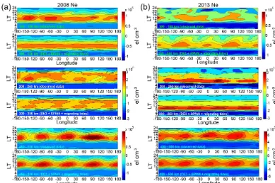
[image:6.612.152.444.360.492.2]Figure 6.2008 September equinox period Ne LT contour plots.(a)LT×longitude maps for electron densities (Ne) for some altitudes of the 50 km interval, during the 2008 September equinox period.(b)Amplitudes obtained for their respective non-migrating tides indicating their frequency (1/day) and respective zonal wavenumber. The corresponding altitude intervals used are indicated in the plots. The color scale, in el cm−3, is shown at the right side of each graph.
The fft2 analysis for the 100–150 km altitude interval indi-cates a large number of waves compared to other altitude in-tervals. This shows that many waves reach the E-region al-titudes, but only some of them are able to disturb the iono-sphere at higher altitudes.
Figure 7 shows the electron density contour plots in dif-ferent altitude intervals observed around the 2013 Septem-ber equinox (left) and their amplitudes. Each graph in Fig. 7 has its own color scale. The DE3 component is present in all the altitude intervals. The SPW4 appears between 100 and 200 km and from 400 to 800 km. Above 500 km only DE3 and SPW4 stand out among the other non-migrating waves. In some altitude intervals it is possible to see DW2 (∼600– 750 km) and SW1 (∼150–600 km) waves. For 2013, DW2 was not observed to be as prominent as in 2008, mainly at al-titudes higher than 500 km. The wave-4 structures are clearly present from∼400 km and above. In the results of the fft2 spectral analysis of amplitudes, the same behavior observed for the 100–150 km altitude interval during 2008 was also ob-served for 2013, indicating that many non-migrating tides’
signatures present in the E-region altitudes could not reach the upper ionosphere.
466 A. N. Onohara et al.: Wavenumber-4 structures observed in the low-latitude ionosphere
Figure 7.2013 September equinox Ne LT contour plots.(a)LT×longitude contour plots for electron density (Ne) for some altitudes of the 50 km interval, during the 2013 September equinox period.(b)Amplitudes obtained for non-migrating tides indicating their frequency (1/day) and respective zonal wavenumber. The corresponding altitude intervals used are indicated in the plots. The color scale, in el cm−3, is shown at the right side of each frame.
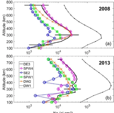
plots showed that in 2008, DW2 had amplitudes close to DE3 and SPW4, and in 2013, the same did not happen. In 2008, SPW1 presented smaller values around the F region peak than in 2013, when its amplitude was largest around 300 km. It can be noticed that the SPW1 signature is more prominent in 2013, while DW2 is more prominent in 2008.
It is important to say that in the graphs of Figs. 6 and 7, the four-peak structures become more evident from ∼250 km, and at higher altitudes, the DE3 and SPW4 waves are of more significance in comparison with other non-migrating waves. Jones et al. (2013) demonstrated that the non-migrating tidal components could be generated in situ in the upper ther-mosphere due to ion–neutral coupling. According to Ober-heide et al. (2011b), DW2 and D0 arise from hydromagnetic coupling between SPW1 and DW1. According to Jones et al. (2013), the hydromagnetic coupling processes affect tidal winds as a result of the Lorentz force in the horizontal mo-mentum equation. For a more complete explanation about this subject, see studies of Richmond (1971) and Forbes and
Garrett (1979). Hagan et al. (2009) showed that the nonlinear interaction between DE3 and DW1 produces SE2 and SPW4. Figures 6, 7, and 8 showed that both DE3 and SPW4 were the most prominent waves in altitudes above the F region peak altitudes. In order to see the importance of DE3 and SPW4 waves in the wave-4 structure formation, we decided to use these waves combined with the diurnal, semidiurnal and terdiurnal migrating tidal modes to build local time ver-sus longitude maps forNmF2,hmF2 and Ne for 2008 and 2013. Ne was plotted for three altitude intervals: 100–150, 200–250 and 400–450 km. These results can be found in Figs. 9, 10 and 11, respectively.
Figure 9 shows the LT×longitude plots obtained for
mi-Figure 8.Amplitudes’ vertical profiles of some waves observed in Figs. 6 and 7. Panel(a)is related to amplitudes observed in the 2008 September equinox period, while(b) is related to those observed in the 2013 equinox period. The same waves’ signatures used in Figs. 3 and 5 were also considered here. DE3, SE2 and SPW4 are supposed to be related to the wave-4 structures in the ionosphere. SPW1 and DW2 are supposed to be related to the offset between the geographic and geomagnetic coordinates. The black horizontal bars on the DE3 plot represent the standard deviation calculated for some altitude intervals.
grating tides were used in the reconstructed plots. Using this type of reconstruction, we intend to see whether it is possi-ble to explain the wave-4 pattern with only these waves. For 2008 the wave-4 pattern is not as pronounced as for 2013. We can conclude that the sum of DE3+SPW4+migrating tides is not enough to explain the wave-4 pattern observed in theNmF2 data in 2008. Other waves were also included in other tests not presented here (DW2, SE2, SPW1), but the plots did not show better results. The plots related to 2013 in Fig. 9 indicated better results than those found for 2008. In the right plots we can easily observe the four peaks in the reconstructed graph. A possibility taken into account is that during high solar periods, the DE3, DW1 and SPW4 absolute amplitudes forNmF2 are higher than those observed during low solar periods. During 2013 it is clear that a combination of DE3, SPW4 and the diurnal, semidiurnal and terdiurnal migrating tides can satisfactorily reproduce the wave-4 struc-tures observed in the data.
Figure 10 shows thehmF2 LT×longitude maps for 2008 (left) and 2013 (right) September equinoxes. Similar to Fig. 9, the upper plots in the Fig. 10 show hmF2 observed previously in Fig. 4, and the bottom plots show their re-spective contour graphs reconstructed using only the sum of DE3+SPW4+migrating tides (diurnal, semidiurnal and terdiurnal). For hmF2, we can observe the wave-4 pattern in reconstructed data for both years 2008 and 2013. This means that the DE3+SPW4+migrating tides are enough
September equinoxes. The upper plots relate to the 100– 150 km interval, the middle plots relate to the 200–250 km interval, and the bottom plots relate to the 450–500 km inter-val. For each altitude interval, we can see the observed data and the reconstructed contour plots using the sum of DE3 +SPW4 +migrating tides. For the 450–500 km interval, both years show good agreement between the observed and reconstructed graphs. This shows that the DE3 and SPW4 modes have great importance at this altitude and that they are the main waves responsible for the wave-4 pattern ob-served. Ne profiles plotted in Fig. 8 showed that this interval was situated above the altitude of the peaks of the main ob-served migrating tides. In the interval of 200–250 km, we can see some similarities between the upper and bottom plots. The agreement is better for 2008 than 2013. In the 100– 150 km interval it can be observed for 2008 that the sum of DE3+SPW4+migrating tides did not result in the wave-4 pattern, meaning that other mechanisms are necessary to ex-plain the four-peak structure observed. Considering the year 2013, the sum resulted in a wave-4 pattern, but did not show a significant similarity with the observed data. For altitudes below the E region, it can be seen in the study of Yue et al. (2010) that a pseudo and reversed-phase wave-4 pattern was evident in the altitudes around E region layers due to the effect of the Abel inversion. Above 800 km the effects due to the plasma drift are weakened.
The results found in this study showed that the wave-4 structures in the ionosphere can be observed in both years of low and high solar activity around September equinoxes. The Ne contour plot showed that the wave-4 structure is not well defined below the ionospheric F-region peak situated around∼300 km. Above this altitude the wave-4 pattern is more clearly visible. Spectral analysis indicated that the main non-migrating waves in the higher altitudes of the ionosphere were the DE3 and SPW4 waves for both years 2008 and 2013. We conclude that these are the main waves responsible for the wave-4 structures seen in the ionosphere.
[image:9.612.76.260.68.249.2]pertur-468 A. N. Onohara et al.: Wavenumber-4 structures observed in the low-latitude ionosphere
Figure 9.Observed and reconstructedNmF2 for 2008 and 2013 around September equinoxes. Panels(a, c)are related to 2008, while(b, d)are related to 2013. Panels(a, b)are the observedNmF2 variation contour plots, also present in Fig. 2. Panels(c, d)were reconstructed using SPW4, DE3 and migrating tide waves’ (DW1, SW2 and TW3) signatures observed in the spectral analysis (not shown) at ionospheric altitudes. The reconstruction done for 2013 clearly shows a wave-4 structure, while the same was not observed for 2008.
Figure 10.Observed and reconstructedhmF2 for 2008 and 2013 around September equinoxes. Panels(a, c)are related to 2008, while(b, d)are related to 2013. Panels(a, b)are the observedhmF2 variation contour plots, also present in Fig. 4. Panels(c, d)were reconstructed using SPW4, DE3 and migrating tide waves’ (DW1, SW2 and TW3) signatures observed in the spectral analysis (not shown) at ionospheric altitudes. Both reconstructions in bottom figures clearly show a wave-4 structure.
bation driven by in situ changes in neutral composition or in the meridional neutral winds; they concluded that the wave-4 structure results from a combination ofE×Bdrifts, neutral winds and neutral composition.
3 Discussion and conclusions
This study has shown that the DE3 wave is the main non-migrating tide responsible for the wave-4 longitude varia-tions observed in satellite data. We also indicated that the wave-4 structure becomes more prominent at altitudes above
250 km, where the DE3 and SPW4 amplitudes were larger than other non-migrating modes. The focus of this work is not related to details about how the wave-4 structures are created in the ionosphere or the mechanisms associated with that, but it is related to investigating which waves are present in these structures and which are the main ones responsible for the four peaks in the longitudinal structure.
[image:10.612.117.478.319.500.2]al-Figure 11.Observed and reconstructed Ne for 2008 and 2013 around September equinoxes. In this figure plots related to the 2008 September equinox period are in(a)panels, while those related to 2013 are in(b)panels. Three intervals were selected: 100–150, 200–250 and 450– 500 km. For each one of these altitude intervals, we show the observed and reconstructed variations. The reconstructions were done using SPW4, DE3 and migrating tide waves’ (DW1, SW2 and TW3) signatures observed in the spectral analysis (not shown) at ionospheric altitudes. The altitude intervals related to each plot in the figure are identified in the plots. The best comparisons were found in the 450– 500 km altitude interval for both years 2008 and 2013.
titudes from∼250 up to∼800 km, it is very clear that the wave-4 structures were caused by these waves via E-region dynamo modulation, consequently affecting the plasma dis-tribution. It is important to mention here that the waves were identified by fft2 analysis, which identified all the waves present in 00:00–24:00 LT and−180 to 180◦distribution.
The diurnal, semidiurnal and sometimes the terdiurnal mi-grating tides usually had the largest amplitudes. The main non-migrating tides identified by the fft2 analysis were plot-ted with their corresponding parameters in this study. Some of these waves were not related to a wave-4 structure, but they have a significant presence, like DW2. This means that more studies are necessary to understand the detailed mech-anisms associated with wave-4 structures in the ionosphere.
In this study we have shown that the wave-4 structures in the equatorial and low-latitude ionospheric parameters can be observed during both low and high solar activity around September equinoxes. These four peaks appeared more prominently in Ne data above F-region peak altitudes. By doing two-dimensional fft2 analysis and selecting some wave signatures to build LT×longitude contour plots, it was verified that the DE3 and SPW4 waves were the main wave modes responsible for this structure in most of the cases.
In the amplitudes calculated from fft2 spectral analysis contour plots, we noticed the presence of DW2, SPW1 and other waves’ signatures not necessarily related to waves of tropospheric origin. SPW1 is related to the offset between the geomagnetic and geographic coordinate, and DW2 is a combination between SPW1 and DW1. DW2 could be ob-served during all the periods selected inhmF2 amplitudes.
NmF2 amplitudes exhibited this wave signature only in pe-riods of high solar activity. DW2 signatures also appeared in Ne fft2 contour plots for both 2008 and 2013 September equinox periods. Vertical amplitude Ne profiles showed that in 2008, DW2 amplitudes were more prominent than in 2013, mainly at altitudes above 250 km. In 2013, SPW1 had larger amplitudes around 300 km.
[image:11.612.99.488.65.324.2]be-470 A. N. Onohara et al.: Wavenumber-4 structures observed in the low-latitude ionosphere
low could reach high altitudes. It is important to keep in mind that the wave-4 structures observed are mainly strongly related to DE3 and SPW4 waves. The detailed way as to how this happens remains unknown. It is possible that the DE3, propagated from lower altitudes by tide modulation to the E region, creating electric fields that combined with thermospheric winds and geomagnetic field lines, gives rise to ionospheric dynamo. The effects caused by this, such as vertical plasma drifts, were possibly responsible for releas-ing tropospheric, thermospheric and geomagnetic influences into higher altitudes of the ionosphere. For the first time, the wave-4 structure over different altitude intervals and two dif-ferent periods of solar cycle activity was investigated. Spec-tral analysis done forNmF2,hmF2 and Ne showed that these structures are mainly related to DE3 and SPW4 waves.
Data availability. The data used in this study are available for download from COSMIC website (www.cosmic.ucar.edu) after reg-istration.
Author contributions. Data analysis and graphics were done by ANO. All the authors made important contributions in the manuscript development.
Competing interests. The authors declare that they have no conflict of interest.
Special issue statement. This article is part of the special issue “Space weather connections to near-Earth space and the atmo-sphere”. It is a result of the 6◦ Simpósio Brasileiro de Geofísica Espacial e Aeronomia (SBGEA), Jataí, Brazil, 26–30 September 2016.
Acknowledgements. Inez Staciarini Batista acknowledges CNPq through grants 474351/2013-0, 4000373/2014-9, 303461/2014-4 and 302920/2014-5 for support. This study was supported by FAPESP, grant number 11/11071-0.
The topical editor, Dalia Buresova, thanks Jaroslav Chum and one anonymous referee for help in evaluating this paper.
References
Abdu, M. A.: Equatorial ionosphere-thermosphere system: Elec-trodynamics and irregularities, Adv. Space Res., 35, 771–787, https://doi.org/10.1016/j.asr.2005.03.150, 2005.
Abdu, M. A.: Electrodynamics of ionospheric weather over low lat-itudes, Geosci. Lett., 3, 11, https://doi.org/10.1186/s40562-016-0043-6, 2016.
Alken, P. and Maus, S.: Spatio-temporal characterization of the equatorial electrojet from CHAMP, Orsted, and
SAC-C satellite measurements, J. Geophys. Res., 112, A09305, https://doi.org/10.1029/2007JA012524, 2007.
Appleton, E. V.: Two anomalies in the ionosphere, Nature, 157, 691, https://doi.org/10.1038/157691a0, 1946.
Batista, I. S. and Abdu, M. A.: Ionospheric variability at Brazil-ian low and equatorial latitudes: comparison between obser-vations and IRI model, Adv. Space Res., 34, 1894–1900, https://doi.org/10.1016/j.asr.2004.04.012, 2004.
Batista, I. S., Diogo, E. M., Souza, J. R., Abdu, M. A., and Bailey, G. J.: Equatorial ionization anomaly: The role of thermospheric winds and effects of the geomagnetic field secular variation, in: Aeronomy of the Earth’s Atmosphere and Ionosphere, edited by: Abdu, M. and Pancheva, D., IAGA Special Sopron Book Series 2, 317–328, Springer, https://doi.org/10.1007/978-94-007-0326-1_23, 2011.
Chang, L. C., Lin, C. H., Yue, J., Liu, J. Y., and Lin, J. T.: Stationary planetary wave and nonmigrating tidal signatures in ionospheric wave 3 and wave 4 variations in 2007–2011 FORMOSAT-3/COSMIC observations, J. Geophys. Res.-Space, 118, 6651– 6665, https://doi.org/10.1002/jgra.50583, 2013.
Ely, C. V., Batista, I. S., and Abdu, M. A.: Radio oc-cultation electron density profiles from the FORMOSAT-3/COSMIC satellites over the Brazilian region: A compari-son with Digicompari-sonde data, Adv. Space Res., 49, 1553–1562, https://doi.org/10.1016/j.asr.2011.12.029, 2012.
Forbes, J. M.: Planetary Waves in the Thermosphere-Ionosphere System, J. Geomagn. Geoelectr., 48, 91–98, https://doi.org/10.5636/jgg.48.91, 1996.
Forbes, J. M.: Dynamics of the Thermosphere, J. Meterol. Soc. Jpn., 85, 193–213, 2007.
Forbes, J. M. and Garrett, H. B.: Theoretical studies of atmospheric tides, Rev. Geophys., 17, 1951–1981, 1979.
Hagan, M. and Forbes, J. M.: Migrating and nonmigrating semidiurnal tides in the upper atmosphere excited by tro-pospheric latent heat release, J. Geophys. Res., 108, 1062, https://doi.org/10.1029/2002JA009466, 2003.
Hagan, M. E., Maute, A., Roble, R. G., Richmond, A. D., Immel, T. J., and England, S. L.: Connections between deep tropical clouds and the Earth’s ionosphere, Geophys. Res. Lett., 34, L201109, https://doi.org/10.1029/2007GL030142, 2007.
Hagan, M. E., Maute, A., and Roble, R. G.: Tropospheric tidal ef-fects on the middle and upper atmosphere, J. Geophys. Res., 114, A01302, https://doi.org/10.1029/2008JA013637, 2009.
Immel, T. J., Sagawa, E., England, S. L., Henderson, S. B. , Hagan, M. E., Mende, S. B., Frey, H. U., Swenson, C. M., and Paxton, L. J.: Control of equatorial ionospheric morphol-ogy by atmospheric tides, Geophys. Res. Lett., 33, L15108, https://doi.org/10.1029/2006GL026161, 2006.
Jones, M. Jr., Forbes, J. M., Hagan, M. E., and Maute, A.: Non-migrating tides in the ionosphere-thermosphere: in situ versus tropospheric sources, J. Geophys. Res.-Space, 118, 2438–2451, https://doi.org/10.1002/jgra.50257, 2013.
nal structure of the equatorial ionosphere: Time evolution of the four-peaked EIA structure, J. Geophys. Res., 112, A12305, https://doi.org/10.1029/2007JA012455, 2007c.
Lin, C. H., Liu, J. Y., Hsiao, C. C., Liu, C. H., Cheng, C. Z., Chang, P. Y., Tsai, H. F., Fang, T. W., Chen, C. H., and Hsu, M. L.: Global ionospheric structure imaged by FORMOSAT-3/COSMIC: early results, Terr. Atmos. Ocean. Sci., 20, 171–179, https://doi.org/10.3319/TAO.2008.01.18.01(F3C), 2009. Liu, G., Immel, T. J., England, S. L., Kumar, K. K., and
Ramkumar, G.: Temporal modulations of the longitudinal structure in F2 peak height in the equatorial ionosphere as observed by COSMIC, J. Geophys. Res., 115, A04303, https://doi.org/10.1029/2009JA014829, 2010.
Liu, H. and Watanabe, S.: Seasonal variation of the longitu-dinal structure of the equatorial ionosphere: Does it reflect tidal influences from below?, J. Geophys. Res., 113, A08315, https://doi.org/10.1029/2008JA013027, 2008.
Lühr, H., Rother, M., Häusler, K., Alken, P., and Maus, S.: The influence of non-migrating tides on the longitudinal variation of the equatorial electrojet, J. Geophys. Res., 113, A08313, https://doi.org/10.1029/2008JA013064, 2008.
Namba, S. and Maeda, K. I.: Radio wave propagation, p. 86, Corona Publishing, Tokyo, 1939 (in Japanese).
Oberheide, J., Forbes, J. M., Zhang, X., and Bruinsma, S. L.: Wave-driven variability in the ionosphere-thermosphere-mesosphere system from TIMED observations: What con-tributes to the “wave 4”?, J. Geophys. Res., 116, A01306, https://doi.org/10.1029/2010JA015911, 2011a.
https://doi.org/10.1029/2010GL044039, 2010.
Pancheva, D. and Mukhtarov, P.: Global Response of the Ionosphere to Atmospheric Tides Forced from Below: Recent Progress Based on Satellite Measurements, Space Sci. Rev., 168, 175–209, https://doi.org/10.1007/s11214-011-9837-1, 2012.
Pedatella, N. M., Hagan, M. E., and Maute, A.: The compara-tive importance of DE3, SE2, and SPW4 on the generation of wavenumber-4 longitude structures in the low-latitude iono-sphere during September equinox, Geophys. Res. Lett., 39, L19108, https://doi.org/10.1029/2012GL053643, 2012. Rishbeth, H.: The equatorial F-layer: progress and puzzles,
Ann. Geophys., 18, 730–739, https://doi.org/10.1007/s00585-000-0730-6, 2000.
Rishmond, A. D.: Tidal winds at ionospheric heights, Radio Sci., 6, 175–189, 1971.
Sagawa, E., Immel, T. J., Frey, U., and Mende, S. B.: Longitudi-nal structure of equatorial anomaly in the nighttime ionosphere observed by IMAGE/FUV, J. Geophys. Res., 110, A11302, https://doi.org/10.1029/2004JA010848, 2005.
Scherliess, L., Thompson, D. D., and Schunk, R. W.: Lon-gitudinal variability of low-latitude total electron con-tent: Tidal influences, J. Geophys. Res., 113, A01311, https://doi.org/10.1029/2007JA012480, 2008.