* Corresponding author. Tel.: +989121784825 ; +989386231359.
E-mail: [email protected] (M. Naderi), [email protected] (M. Naderi) © 2013 Growing Science Ltd. All rights reserved.
doi: 10.5267/j.ijiec.2013.02.002
International Journal of Industrial Engineering Computations 4 (2013)191–202 Contents lists available at GrowingScience
International Journal of Industrial Engineering Computations
homepage: www.GrowingScience.com/ijiec
An imperialist competitive algorithm for a bi-objective parallel machine scheduling problem with load balancing consideration
Mansooreh Madani-Isfahania, Ehsan Ghobadiana, Hassan Irani Tekmehdashc,d, Reza Tavakkoli-Moghaddamb and Mahdi Naderi-Benia*
aDepartment of Industrial Engineering, South Tehran Branch, Islamic Azad University, Tehran, Iran
bDepartment of Industrial Engineering, College of Engineering, University of Tehran, Tehran, Iran
cDepartment of Transportation Engineering, Islamic Azad University, Science and Research Branch, Tehran, Iran
dDepartment of Construction Management, Islamic Azad University, Science and Research Branch, Tehran, Iran
C H R O N I C L E A B S T R A C T
Article history:
Received October252012 Received in revised format December 28 2012
Accepted February4 2013 Available online 6February2013
In this paper, we present a new Imperialist Competitive Algorithm (ICA) to solve a bi-objective unrelated parallel machine scheduling problem where setup times are sequence dependent. The objectives include mean completion time of jobs and mean squares of deviations from machines workload from their averages. The performance of the proposed ICA (PICA) method is examined using some randomly generated data and they are compared with three alternative methods including particle swarm optimization (PSO), original version of imperialist competitive algorithm (OICA) and genetic algorithm (GA) in terms of the objective function values. The preliminary results indicate that the proposed study outperforms other alternative methods. In addition, while OICA performs the worst as alternative solution strategy, PSO and GA seem to perform better.
© 2013 Growing Science Ltd. All rights reserved Keywords:
Parallel machine scheduling Genetic algorithm
Imperialist competitive algorithm Load Balancing
Particle swarm optimization
1. Introduction
Rajakumar et al. (2004) presented a method where workflow and workload were assumed to have the same meaning and a machine with the lowest workflow is chosen for assignment of a new job from the list of unfinished jobs. They considered various priority strategies for the selection of jobs and three various strategies were considered, namely random (RANDOM), shortest processing time (SPT) and longest processing time (LPT) for the selection of jobs for workflow balancing. The relative percentage of imbalance (RPI) was chosen among the parallel machines to assess the performance of these strategies in a standard manufacturing environment.
T'kindt et al. (2001) considered a bicriteria scheduling problem connected with the glass bottles production where the shop was made up of unrelated parallel machines and the aim was to compute a schedule of orders, which maximizes the total margin and minimizes the difference in machines workload. Rajakumar et al. (2004), in another assignment, implemented genetic algorithm (GA) to solve the parallel machine scheduling problem of the manufacturing system with the objective of workflow balancing. They compared the performance of GA with three workflow balancing strategies namely RANDOM, SPT and LPT. They adopted RPI among parallel machines for assessing the performance of these heuristics and reported that GA provided better performance for the combination of different job sizes and machines.
Keskinturk et al. (2012) investigated the problem of minimizing average relative percentage of imbalance (ARPI) with sequence-dependent setup times in a parallel-machine environment. They presented a mathematical model, which minimizes ARPI, used some heuristics, and two metaheuristics, an ant colony optimization algorithm and a GA, and examined on different random data. Their method provided better results using ant colony optimization than heuristics and GA did.
Ho et al. (2009) proposed another method for minimizing the normalized sum of square for workload deviations on m parallel processors called normalized sum of square for workload deviations (NSSWD). Vallada and Ruiz (2011) presented GA for the unrelated parallel machine scheduling problem where machine and job sequence dependent setup times were considered and their results seemed to provide an excellent performance overcoming the rest of the evaluated techniques in a comprehensive benchmark set of instances.
Varmazyar and Salmasi (2012) considered flow shop scheduling problems with sequence-dependent setup times, minimizing the number of tardy jobs, and proposed a mixed integer programming to solve the resulted problem. They also proposed several meta-heuristic methods based on tabu search (TS) and ICA to heuristically solve the problem. They reported that the performance of ICA was worse than the other algorithms for some small and medium sized instances while the hybrid of ICA and the TS algorithm provided better performance than the other proposed algorithms for large-sized problems.
Tavakkoli-Moghaddam et al. (2009) presented two-level mixed-integer programming model of scheduling N jobs on M parallel machines, which minimizes bi-objectives, namely the number of tardy jobs and the total completion time of all the jobs and with unrelated parallel machines. They used GA to solve the bi-objective parallel machine scheduling problem and the performance of the proposed model and GA was verified using various instances. Shokrollahpoura et al. (2009) considered two-stage assembly flowshop scheduling problem with minimization of weighted sum of makespan and mean completion time as the objective and used ICA to solve the resulted problem. Raghavendra et al. (2006) investigated workflow balancing in parallel machine scheduling with precedence constraints using GA.
that the proposed two-phase model of this paper performed relatively better than Zimmerman's single-phase fuzzy method. Moradinasab et al. (2011) provided a no-wait two-stage flexible flow shop scheduling problem with setup times where the objective function was to minimize the total completion time. The problem was solved using an AICA and GA. Lian (2010) presented united search particle swarm optimization algorithm for multiobjective scheduling problem while Keskinturk et al. (2012) considered an ant colony optimization algorithm for load balancing in parallel machines with sequence-dependent setup times. Karimi et al. (2011) investigated group scheduling in flexible flow shops by considering a hybridized approach of ICA and electromagnetic-like mechanism and Jolai et al. (2012) studied a novel hybrid meta-heuristic algorithm for a no-wait flexible flow shop scheduling problem with sequence dependent setup times. Javadi et al. (2008) investigated no-wait flow shop scheduling using fuzzy multi-objective linear programming.
In this paper, we present an ICA to solve a bi-objective unrelated parallel machine scheduling problem where setup times are sequence dependent. The objectives include mean completion time of jobs and mean squares of deviations from machines workload from their averages. The performance of the proposed ICA (PICA) method is examined using some randomly generated data and they are compared with three alternative methods including particle swarm optimization (PSO), original version of imperialist competitive algorithm (OICA) and genetic algorithm (GA) in terms of the objective function values.
2. The proposed model
In this study, we consider a mathematical model for ̅,∑( ) , which was originally developed by Keskinturk et al. (2012), where j and k represent indexes associated with jobs, which are integer numbers between one to n+m. Without loss of generality, we assume jobs 1 to n are real and jobs n+1 to n+m are dummy ones with zero processing and setup times, where m is the number of unrelated parallel machines. In addition, the setup time of the first job processed after a dummy job is assumed to be initial setup time. Finally, there is a dummy job on each machine at the beginning of sequencing. The following summarizes the necessary notations for the proposed model of this paper,
ji
p Processing time of job j on machine i
jik
s Setup time of machine i for processing job k after job j
i
w Workload of machine i
w The average workload, i.e.
1 /
m i i
w w m
=
=
∑
j
C Completion time of job j
C The average completion time, i.e.
1 /
n j j
C C n
=
=
∑
ji
Y Binary variable where it is one if job j is processed on machine i and zero, otherwise,
jik
X Binary variable where it is one if job k is processed after job j on machine i and zero, otherwise,
The proposed model of this paper is as follows,
(1)
min = ̅ =∑
(2) min =∑ ( − )
− 1
(3) ∀ ≥ + 1
= 1 (4) ∀ , ≠ ≤ 1 (5) ∀ , , ≠ ≤ (6) ∀ , ≤ , ≠ = (7) ∀ = 1 (8) ∀ = 1 (9) ∀ ≥ + 1
= 0
(10) ∀ , , , ≠
+ 1 − ≥ + +
(11) ∀ , ≠ = + (12) ∀ , , , ≠
, ∈ {0,1}
Here, Eq. (1) and Eq. (2) represent mean completion time and mean squares of workloads from their average. Eq. (3) assigns one dummy job to each machine and guarantees that all dummy jobs are processed at the beginning of operations for each machine. According to Eq. (4), only one job is processed once each machine is available. Eq. (5) guarantees that only one real job can be processed when a machine becomes available. According to Eq. (6), when the processed of a particular job is completed, there is a real or dummy job before. Eq. (7) is used to assure that each job is assigned only to one machine, Eq. (8) assures that one machine cannot process more than one job at the same time, Eq. (9) guarantees that completion times of dummy jobs are equal to zero. In addition, Eq. (10) shows the relationship between two consecutive jobs, Eq. (11) computes the workload of each machine and Eq. (12) demonstrates the variable type.
3. Solution method
The proposed solution strategy of this paper uses two parameters of α and β to merge two objective functions, ̅,∑( ) , into single one ̅ + ∑( ) where α+β=1. The proposed metaheuristics uses a string with the size of n+m-1 where n represents the number of jobs, m denotes the number of machines, and the feasible solutions are integer numbers between one and n+m-1, which is design using the proposed method by Lian (2010). For instance, Fig. 1 demonstrates a sample of jobs and machines when there are three machines and ten jobs.
12 11 10 9 8 7 6 5 4 3 2 1 0.18 0.29 0.35 0.27 0.30 0.08 0.07 0.26 0.32 0.39 0.81 0.96
Sort real numbers↓
1 2 3 10 4 8 11 9 5 12 7 6 0.96 0.81 0.39 0.35 0.32 0.30 0.29 0.27 0.26 0.18 0.08 0.07
Convert real numbers to integer ones↓
1 2 3 10 4 8 * 9 5 * 7 6 Decode
1: 6 → 7 2: 5 → 9 3: 8 → 4 → 10 → 3 → 2 → 1
Termination criterion is the number of function evaluation (NFE) and since we intend to compare the performance of the proposed method with other methods, we use this criterion to have a fair comparison.
3.1. Particle swarm optimization
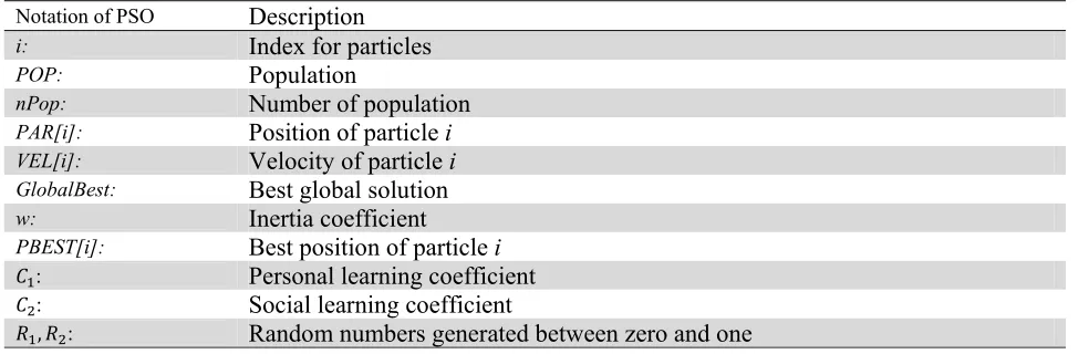
Particle swarm optimization (PSO) has been a popular method, which uses a swarm intelligence to find best solution (Kennedy & Eberhart, 1995). For PSO implementation, we use the following notations,
Table 1
Description Notation of PSO
Index for particles
i:
Population
POP:
Number of population
nPop:
Position of particle i
PAR[i]:
Velocity of particle i
VEL[i]:
Best global solution
GlobalBest:
Inertia coefficient
w:
Best position of particle i
PBEST[i]:
Personal learning coefficient :
Social learning coefficient :
Random numbers generated between zero and one
, :
The following steps are used to apply PSO for the proposed method of this paper,
Initialization
Step 1. Choose initial values,
Step 2. Setup initial values using some randomly generated data for all particles with zero value for velocity,
Step 3. Decode the solution and compute the combined objective function based on ̅ + ∑( ) ,
Step 4. Choose the particles with minimum cost and store its position as GlobalBest,
Step 5. Choose the best personal position
Repeat steps 6 to 12 until termination criterion is met.
Step 6. Update velocity using Eq. (13) as follows,
(13)
[ ]( ) = . [ ]( ) + . ( [ ] − [ ]) + . ( − [ ])
Step 7. Update each particle position based on Eq. (14)
(14)
Step 8. Similar to what we have done in step 3, evaluate position of each particle, update the
best position of each particle and determine the best global solution.
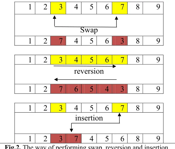
Step 9. Do a local search using of the three methods of Swap, Reversion and Insertion with
equal probabilities as shown in Fig. 2.
9
8
7
6
5
4
3
2
1
Swap
9
8
3
6
5
4
7
2
1
9
8
7
6
5
4
3
2
1
reversion
9
8
3
4
5
6
7
2
1
9
8
7
6
5
4
3
2
1
insertion
9
8
6
5
4
7
3
2
1
Fig.2. The way of performing swap, reversion and insertion
Step 10. If the local search yields better solution, replace it with current solution, and update
the best position of each particle
Step 11. Update the best global solution,
Step 12. Do a local search on GlobalBest and update current solution.
3.2. Genetic algorithm
The proposed genetic algorithm (Holland, 1975; Goldberg, 1989) of this paper has the following steps,
Table 2 demonstrates the GA parameters
Table 2
Description Notation of GA
Member of population
POP[i]:
Population number
nPop:
Portion of population used for crossover operation
pCrossover:
Number of parents for crossover operation
nCrossover:
Portion of mutation
pMutation:
Number of mutation
nMutation:
Mutation ratio
mu:
Number of genes from a chromosome for mutation
nmu:
Tournament size
TournamentSize:
A number between zero and one
The GA used for the proposed model of this paper is a standard method adopted from
Haupt and Haupt (2004) and it is briefly described here,Step 1. Setup all input parameters,
Step 2. Position all individuals,
Step 3. Evaluate each position,
Step 4. Order population in non-decreasing order according to their objective functions,
Repeat step 5 to 7 until termination criterion is met
Step 5. Perform crossover based on the following,
(15)
= 2 ∗ ( .
2 )
Let X1 and X2be the parents and Y1 and Y2be the children. We generate X1 and X2randomly in the
interval of [− , 1 + ] and Y1 and Y2are generated as follows,
(16)
= . + (1 − ).
(17)
= . + (1 − ).
Step 6. Perform mutation based on nMutation
(18)
= ( . )
The mutation operation is similar to Engelbrecht (2007), as follows
(19)
= 0.5 ∗ ( − )
(20)
= + .
Step 7. Merge the initial population with two new populations obtained from mutation and crossover and order them on non-decreasing order,
(18)
= ( . )
Step 8. Choose the first nPop components as new solution.
3.3 Proposed Imperialist Competitive Algorithm
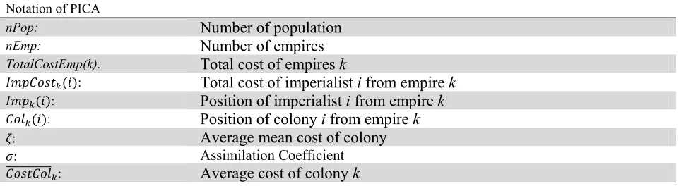
In this section, we present details of the proposed imperialist competitive algorithm (PICA), which is originally presented by Atashpaz-Gargari and Lucas (2007).Table 3 demonstrates details of parameters used,
Table 3 Notation of PICA
Number of population
nPop:
Number of empires
nEmp:
Total cost of empires k
TotalCostEmp(k):
Total cost of imperialist i from empire k
( ):
Position of imperialist i from empire k
( ):
Position of colony i from empire k
( ):
Average mean cost of colony :
Assimilation Coefficient :
Average cost of colony k
The following summarizes the necessary steps associated with the proposed study,
Step 1. Setup initial values,
Step 2. Determine empires (Similar to step 2 of GA and PSO),
Step 3. Order countries based on their costs in non-decreasing orders and based on nEmp and nPop-nEmp assign countries to Imperialists. The assignment of countries to Imperialists are performed based
on pi calculated using Boltzmann (Engelbrecht, 2007) and roulette wheel selection strategy as follows,
(21) , =
. ( )
( ( ))
(22) =
,
∑ ,
where η is the pressure coefficient. Total cost associated with empire k is also calculated as follows,
(23)
( ) = s ( ) + . .
Repeat steps 5 to 10 until termination criterion is met,
Step 5. Go inside each empire, do Assimilation on all colonies and calculate new location as follows,
(24)
Col ( )( ) = ( )( ) + . . ( ) − ( )( ) .
In Eq.(24), r is a string whose elements are generated randomly between zero and one.
Step 6. Do revolution on each Empire and its colonies,
To do this, we first perform a local search on each Imperialist and of the new location maintain a better objective function, replace the new position with the old one. This policy is applied to all colonies and the positions are updated, accordingly.
Step 7. If the position of colonies is better than its Empire in terms of their costs, exchange their position,
Step 8. Update empire cost using Eq. (23),
Step 9. Choose the worst Empire in terms of cost and assign its worst colony to other Empire,
Step 10. Perform a local search on the best Empire.
4. The results
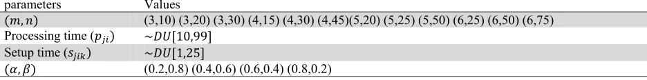
In this section, we examine the performance of the proposed method of this paper on some randomly generated data. Table 4 shows the input data,
Table 4
The way of generating input parameters Values
parameters
(3,10) (3,20) (3,30) (4,15) (4,30) (4,45)(5,20) (5,25) (5,50) (6,25) (6,50) (6,75)
( , )
~ [10,99]
Processing time ( )
~ [1,25]
Setup time ( )
(0.2,0.8) (0.4,0.6) (0.6,0.4) (0.8,0.2)
We have performed different studies to find the best tuning values. The likelihood of a revolution is considered as 0.05 with the rate of 0.05. The value of NFE for problems 3, 4, 5 and 6 are 100000, 150000, 200000 and 250000, respectively. Table 5 demonstrates some other parameters,
Table 5
The values of parameters of GA, PSO and PICA
PICA PSO
GA
nPop=150 nPop=100
nPop=100
nEmp=15 w=0.3
pCrossover=0.8
= 1 = 0.8
pMutation=0.1
= 1.7 = 1
mu=0.05
= 0.1
TournamentSize=3
Each example is solved 5 times leading us to have 960 instances, we have considered various values for
α, and β. Table 6, Table 7, Table 8 and Table 9 demonstrate the results of our survey.
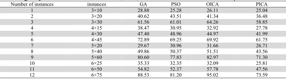
Table 6
The average objective function values of GA, PSO, OICA and PICA while α=0.2 and β=0.8
Number of instances
instances GA PSO OICA PICA
1 3×10 28.88 25.28 26.11 25.04
2
3×20 40.62 43.51 41.34 36.48
3 3×30 61.56 61.01 64.26 58.85
4
4×15 38.47 30.95 32.92 27.78
5 4×30 47.40 48.96 44.97 41.99
6
4×45 72.89 69.25 69.92 61.75
7 5×20 29.67 30.96 31.66 26.71
8
5×40 49.86 50.37 51.51 43.56
9 5×60 80.60 77.83 82.97 71.30
10
6×25 35.33 32.35 32.09 25.81
11 6×50 54.82 52.37 57.78 47.56
12
6×75 88.53 81.20 95.02 73.59
Table 7
The average objective function values of GA, PSO, OICA and PICA while α=0.4 and β=0.6
Number of instances
instances GA PSO OICA PICA
1 3×10 53.75 51.49 50.09 43.43
2
3×20 74.58 69.01 77.89 75.14
3 3×30 119.18 119.49 121.86 112.25
4
4×15 78.19 60.00 54.64 49.46
5 4×30 86.41 85.02 92.55 80.89
6
4×45 137.06 128.41 139.02 125.10
7 5×20 56.92 57.80 55.97 47.92
8
5×40 96.97 92.38 95.19 86.31
9 5×60 154.08 143.06 163.37 135.88
10
6×25 56.81 55.92 62.01 50.31
11 6×50 102.51 107.85 111.54 91.83
12
6×75 169.80 165.63 172.26 143.49
Table 8
The average objective function values of GA, PSO, OICA and PICA while α=0.6 and β=0.4
Number of instances
instances GA PSO OICA PICA
1 3×10 74.30 68.41 77.52 66.99
2
3×20 110.37 102.55 111.89 102.12
3 3×30 172.65 165.34 174.35 164.45
4
4×15 99.92 90.21 83.47 79.68
5 4×30 124.54 124.89 126.05 113.31
6
4×45 199.14 191.78 202.08 175.56
7 5×20 87.94 89.91 81.31 74.28
8
5×40 137.47 138.48 138.59 122.84
9 5×60 226.74 238.72 221.71 194.47
10
6×25 88.98 90.74 79.79 70.27
11 6×50 135.57 158.60 164.49 134.85
12
Table 9
The average objective function values of GA, PSO, OICA and PICA while α=0.8 and β=0.2
Number of instances
instances GA PSO OICA PICA
1 3×10 94.56 85.31 90.76 84.76
2
3×20 143.25 124.32 145.04 123.71
3 3×30 217.50 198.77 224.28 196.08
4
4×15 112.57 103.87 96.51 84.80
5 4×30 158.47 159.61 151.41 136.26
6
4×45 239.36 255.60 269.46 216.95
7 5×20 107.72 107.67 107.44 89.71
8
5×40 179.94 173.12 179.38 148.27
9 5×60 279.86 289.52 312.13 247.38
10
6×25 105.69 103.84 104.99 90.15
11 6×50 200.87 189.67 200.96 157.01
12
6×75 286.70 300.32 348.02 264.82
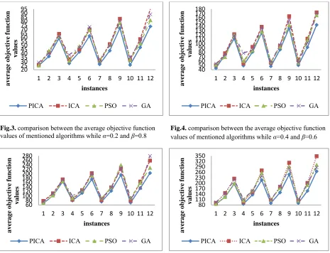
In addition, we present the results in terms of descriptive figures and Fig. 3 to Fig. 5 show the results.
Fig.4. comparison between the average objective function values of mentioned algorithms while α=0.4 and β=0.6 Fig.3. comparison between the average objective function
values of mentioned algorithms while α=0.2 and β=0.8
Fig.6. comparison between the average objective function values of mentioned algorithms while α=0.8 and β=0.2 Fig.5. comparison between the average objective function
values of mentioned algorithms while α=0.6 and β=0.4
As we can observe from the results of Fig. 3 to Fig. 6, PICA performs better than other alternative methods including ICA, PSO and GA, especially when the sizes of instances increase. ICA performs the worst while GA and PSO come somewhere between.
40 50 60 70 80 90 100 110 120 130 140 150 160 170 180
1 2 3 4 5 6 7 8 9 10 11 12
ave rage obje ctive fu nc ti on va lu es instances
PICA ICA PSO GA
20 25 30 35 40 45 50 55 60 65 70 75 80 85 90 95
1 2 3 4 5 6 7 8 9 10 11 12
ave rage obje ctive fu nc ti on va lu es instances
PICA ICA PSO GA
80 110 140 170 200 230 260 290 320 350
1 2 3 4 5 6 7 8 9 10 11 12
av er age objective fu nc ti on valu es instances
PICA ICA PSO GA
60 80 100 120 140 160 180 200 220 240 260 280
1 2 3 4 5 6 7 8 9 10 11 12
av er age objective fu nc ti on valu es instances
5. Conclusion
In this paper, we have presented a new Imperialist Competitive Algorithm (ICA) to solve a bi-objective unrelated parallel machine scheduling problem where setup times are sequence dependent. The objectives include mean completion times of jobs and mean squares of deviations from machines workload from their averages. The performance of the proposed ICA (PICA) method has been examined using some randomly generated data and they have been compared with three alternative methods including particle swarm optimization (PSO), original version of imperialist competitive algorithm (OICA) and genetic algorithm (GA) in terms of the objective function values. The preliminary results have indicated that the proposed study outperforms other alternative methods. In addition, while OICA performs the worst as alternative solution strategy, PSO and GA seem to perform better.
References
Allahverdi, A., Ng, C., Cheng, T., & Kovalyov, M. (2008).A survey of scheduling problems with setup times or costs.European Journal of Operational Research, 187, 985-1032.
Atashpaz-Gargari, E., & Lucas, E. C. (2007). Imperialist Competitive Algorithm: An algorithm for optimization inspired by imperialist competitive.IEEE Congress on Evolutionary Computation,
Singapore, 4661-4667.
Cossari, A., Ho, J.C., Paletta, G., &Torres, A.J.R. (2012).A new heuristic for workload balancing on identical parallel machines and a statistical perspective on the workload balancing criteria,
Computers and Operations Research, 39, 1382-1392.
Engelbrecht, A. P. (2007). Computational Intelligence: An Introduction, 2nd ed., Wiley.
Goldberg, D.E. (1989). Genetic Algorithms in Search, Optimization and Machine Learning. Addison Wesley Longman.
Haupt, R. L., & Haupt, S. E. (2004).Practical Genetic Algorithm.2nd ed., Wiley.
Ho, J.C., Tseng, T.L.B., Torres, A.J.R., Lopez, F.J. (2009).Minimizing the normalized sum of square for workload deviations on m parallel processors.Computers and Industrial Engineering, 56, 186-192.
Holland, J.H. (1975).Adaptation in Natural and Artificial Systems. University of Michigan Press, Ann Arbor.
Hoogeveen, H. (2005). Multicriteria scheduling. European Journal of Operational Research, 167, 592-623.
Javadi, B., Saidi-Mehrabad, Haji, A., Mahdavi, I., Jolai, F., & Mahdavi-Amiri, N. (2008).No-wait flow shop scheduling using fuzzy multi-objective linear programming.Journal of Franklin Institute, 345, 452-467.
Jolai, F., Rabiee, M., & Asefi, H. (2012). A novel hybrid meta-heuristic algorithm for a no-wait flexible flow shop scheduling problem with sequence dependent setup times.International Journal of
Production Research, 50 (24), 7447-7466.
Karimi, N., Zandieh. M., & Najafi, A. A. (2011). Group scheduling in flexible flow shops: a hybridised approach of imperialist competitive algorithm and electromagnetic-like mechanism.International
Journal of Production Research, 49 (6), 4965-4977.
Kennedy, J., & Eberhart, R.C. (1995).Particle swarm optimization.In: Proceedings of the 1995 IEEE
International Conference on Neural Networks, 4, 1942-1948.
Keskinturk, T., Yildirim, M.B., & Barut, M. (2012). An ant colony optimization algorithm for load balancing in parallel machines with sequence-dependent setup times.Computers & Operations
Research, 39, 1225-1235.
Lei, D. (2009). Multi-objective production scheduling: a survey.International Journal of Advanced
Manufacturing Technology, 43(9-10), 926-938.
Moradinasab, N., Shafaei, R., Rabiee, M., & Ramezani, P. (2012). No-wait two stage hybrid flowshop scheduling with genetic and adaptive imperialist competitive algorithms.Journal of Experimental &
Theoretical Artificial Intelligence, DOI: 10.1080/0952813X.2012.682752.
Naderi-Beni, M., Tavakkoli-Moghaddam, R., Naderi, B., Ghobadian, E., & Pourrousta, A. (2012). A two-phase fuzzy programming model for a complex bi-objective no-wait flow shop scheduling.
International Journal of Industrial Engineering Computations, 3, 617-626.
Nagar, A., Haddock, J., Heragu, S. (1995). Multiple and bicriteria scheduling: a literature survey.
European Journal of Operational Research, 81, 88-104, DOI: 10.1016/0377-2217(93) E0140-S.
Ouazene, Y., Hnaien, F., Yalaoui, F., & Amodeo, L. (2011). The joint load balancing and parallel machine scheduling problem.Operations Research Proceedings 2010, DOI:
10.1007/978-3-642-2009-0_79, Springer_Verlag Berlin Heidelberg.
Pinedo, M.L. (2008). Scheduling, Algorithms, and Systems.3rd ed., Springer.
Raghavendra, B.V., & Murthy, A.N.N. (2011).Workload balancing in identical parallel machine scheduling while planning in flexible manufacturing system using genetic algorithm.ARPN Journal
of Engineering and Applied Sciences, 6 (1).
Rajakumar, S., Arunachalam, V.P., & Selladurai, V. (2004). Workflow balancing strategies in parallel machine scheduling.International Journal of Advanced Manufacturing Technology, 23, 366-374, DOI: 10.1007/s00170-003-1603-4.
Rajakumar, S., Arunachalam, V.P., & Selladurai, V. (2006).Workflow balancing in parallel machine scheduling with precedence constraints using genetic algorithm.Journal of Manufacturing
Technology Management, 17, 239-254.
Rajakumar, S., Arunachalam, V.P., & Selladurai, V. (2007).Workflow balancing in parallel machines through genetic algorithm.International Journal of Advanced Manufacturing Technology, 33, 1212-1221, DOI: 10.1007/s00170-006-0553-z.
Shokrollahpour, E., Zandieh, M., & Dorri, B. (2011).A novel imperialist competitive algorithm for bi-criteria scheduling of the assembly flowshop problem.International Journal of Production Research, 49 (11), 3087-3103.
Tavakkoli-Moghaddam, R., Taheri, F., Bazzazi, M., Izadi, M., & Sassani, F. (2009). Design of a genetic algorithm for bi-objective unrelated parallel machines scheduling with sequence-dependent setup times and precedence constraints.Computers and Operations Research, 36, 3224-3230.
T’Kindt, V., Billaut, J.C., & Proust, C. (2001).Solving a bicriteria scheduling problem on unrelated parallel machines occurring in the glass bottle industry.European Journal of OperationalResearch, 135, 42-49.
Vallada, E., & Ruiz, R. (2011). A genetic algorithm for the unrelated parallel machine scheduling problem with sequence dependent setup times.European Journal of Operational Research, 211, 612-622.
Varmazyar, M., & Salmasi, N. (2012).Sequence-dependent flow shop scheduling problem minimising the number of tardy jobs.International Journal of Production Research, 50 (20), 5843-5858.