DEMOGRAPHIC RESEARCH
VOLUME 33, ARTICLE 13, PAGES 363
−
390
PUBLISHED 26 AUGUST 2015
http://www.demographic-research.org/Volumes/Vol33/13/ DOI: 10.4054/DemRes.2015.33.13
Research Material
Average age at death in infancy and infant
mortality level: Reconsidering the
Coale-Demeny formulas at current levels of low
mortality
Evgeny M. Andreev
W. Ward Kingkade
©2015 Evgeny M. Andreev & W. Ward Kingkade.
This open-access work is published under the terms of the Creative Commons Attribution NonCommercial License 2.0 Germany, which permits use, reproduction & distribution in any medium for non-commercial purposes, provided the original author(s) and source are given credit.
1 Introduction 364
2 Data and methods 367
2.1 Methods of calculating average age of death in infancy 367
2.2 Data 368
3 Results 370
4 Discussion 378
5 Conclusion 380
6 Acknowledgements 381
References 382
Appendix 1 385
Appendix 2 387
Average age at death in infancy and infant mortality level:
Reconsidering the Coale-Demeny formulas at current levels of low
mortality
Evgeny M. Andreev1
W. Ward Kingkade2
Abstract
BACKGROUND
The long-term historical decline in infant mortality has been accompanied by increasing concentration of infant deaths at the earliest stages of infancy. In the mid-1960s Coale and Demeny developed formulas describing the dependency of the average age of death in infancy on the level of infant mortality, based on data obtained up to that time.
OBJECTIVE
In the more developed countries a steady rise in average age of infant death began in the mid-1960s. This paper documents this phenomenon and offers alternative formulas for calculation of the average age of death, taking into account the new mortality trends.
METHODS
Standard statistical methodologies and a specially developed method are applied to the linked individual birth and infant death datasets available from the US National Center for Health Statistics and the initial (raw) numbers of deaths from the Human Mortality Database.
RESULTS
It is demonstrated that the trend of decline in the average age of infant death becomes interrupted when the infant mortality rate attains a level around 10 per 1000, and modifications of the Coale-Demeny formulas for practical application to contemporary low levels of mortality are offered.
1 Corresponding author. The Center for Demographic Research, The New Economic School, Moscow,
Russia. E-Mail: [email protected].
CONCLUSIONS
The average age of death in infancy is an important characteristic of infant mortality, although it does not influence the magnitude of life expectancy. That the increase in average age of death in infancy is connected with medical advances is proposed as a possible explanation.
1. Introduction
During the period from the 1920s to the 1970s, infant mortality decline in Europe and other industrialized countries was accompanied by a concentration of infant deaths in the neonatal period. The distribution of infant deaths became more and more highly skewed. The average length of life for infants who died during the first year in low-mortality countries was less than 0.25 years and exhibited systematic decline as the infant mortality rate (IMR) decreased.
The average duration until death for infants who die is an important parameter in life table construction. It is used for the calculation of infant mortality rates from infant death rates and other life table functions at age 0, especially if Chiang’s simple formula (Chiang 1978) is employed. Where direct data on the average age of death in infancy are not available, a set of formulas known as the Coale-Demeny formulas (C-D formulas) that describe the relation between the infant mortality rate and the average age of infant death, 1
a
0, have been the most widely used to estimate1a0from 1q0. In the 1980s the C-D formulas were included in the UN software package for mortality measurement, MORTPAK (1988). In 2001 it was advocated as the basic formula for calculation of the average age of infant death and for calculation of 1q0based on1M0 (Preston, Heuveline, and Guillot 2001:47). Finally, it was a basic formula employed in the Human Mortality Database (HMD) (Wilmoth et al. 2007) that was launched in May 2002. The C-D formulas continue to be recommended in textbooks for calculation of0 1a .
(or MORTPAK) and do not accept any arbitrary estimate of 1a0 (for example, in all official life tables for France, 1a0 is equal to ½; hence we exclude France).
To be specific, the C-D formula indicates that if 1q0 <0.011 the average age of infant death for both males and females is less than 0.8 months. However, in the US life tables for the period 2000 and after, with 1q0<0.008 (Arias, Rostron, and Tejada-Vera 2010), the average age of infant death exceeds 1.3 months. In Japan (2007)3, with
0
1q =0.00274 for males and 0.00244 for females, the average age of infant death is
more than 2 months. In the Human Life Table Database (HLD)4 we found 277 national-level life tables for 23 countries or regions (Australia, Austria, Canada, Chile, Cuba, Germany, Greece, Hong Kong, Hungary, Ireland, Italy, Japan, New Zealand, Poland, Portugal, Singapore, Slovenia, Spain, Taiwan, United States of America) with male infant mortality rates less than 0.010 that have been published with all the details needed to estimate the exact value of average age of infant death, 1a0. In all these life tables except those for Italy, the average age of infant death is more than 1 month.
The number of countries using C-D formulas is small. However, the C-D formulas are important elements of MORTPAK, which is used in all calculations of the Population Division of the UN Department of Economic and Social Affairs. Global analyses need to use a unified methodology, and international databases such as HMD or HLD widely use the C-D formulas. Application of the C-D formulas does not appreciably distort most of the life table indicators and has almost no effect on life expectancy at birth. Nevertheless, the presence in a life table of an indicator that is known to be incorrect seems undesirable to us. Indiscriminate use of the C-D formulas contributes to the dissemination of misinformation about the dependence of the average age of death in infancy on the infant mortality level.
The history of the C-D formulas is as follows. In the early 1960s, Ansley J. Coale and Paul Demeny developed for their influential series of regional model life tables an algorithm for calculating 1a0, the average age of death in age interval (0,1) for infants who died in the interval (1966:(20)). This important parameter is necessary for beginning the life table. The number of person-years lived in the interval from birth to exact age 1,1L0, is related to l1, the number of survivors to age 1, and l0, the hypothetical number of births, by the actuarial relation1L0=1a0⋅l0+(1−1a0)⋅l1, which leads in turn to the following formula for deriving the infant mortality rate,1q0, from the death rate observed in the age interval from 0 to 1, 1m0:
0 1 0 1
0 1 0
1
) 1 (
1 a m
m q
⋅ − +
= .
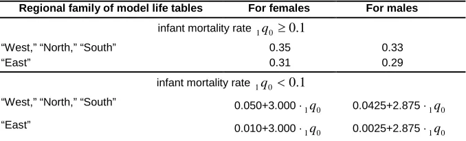
Table 1: Ansley J. Coale and Paul Demeny formulas for estimation of average
age of death in infancy based on the infant mortality rate q 0
Regional family of model life tables For females For males
infant mortality rate 1q0 ≥0.1
“West,” “North,” “South” 0.35 0.33
“East” 0.31 0.29
infant mortality rate 1q0 <0.1
“West,” “North,” “South” 0.050+3.000 ·
0
1q 0.0425+2.875 ·1q0
“East” 0.010+3.000 ·
0
1q 0.0025+2.875 ·1q0
Note: Coale and Demeny denoted average age of death in the age interval 0-1 by k0, but we have adopted an alternative notation.
These formulas for 1
a
0 were a minor detail within the Coale-Demeny system of model life tables, which has been variously employed to describe relations between levels of fertility and mortality on the one hand and population structure on the other hand, and which has been widely applied in demographic analysis of Third World countries lacking reliable vital statistics, as well as in historical demography of European populations. Somewhat ironically, the formulas for 1a
0 seem to have found more widespread use than the model life table system itself, being employed in the construction of life tables for many analyses that have not otherwise involved the model life tables.In the 1970s, related formulas were developed for calculating average age of infant death based on the central death rate at age 0: 1M0(Arriaga, Anderson, and Heligman 1976). They used only the higher (for regions “West”, “North”, “South”) variant of the formula for each sex separately. These formulas became known as the “Coale Demeny formulas” and have been widely used ever since.
individual birth and infant death records available from the National Center for Health Statistics of the U.S. Centers for Disease Control and Prevention, we seek to explain why major infant mortality declines can be combined with relatively high ages of infant death.
2. Data and methods
2.1 Methods of calculating average age of death in infancy
For precise computation of the average age of infant death it is necessary to have either the aggregate distribution of deaths by age in great detail (e.g., days), or, at a minimum, in days during the first month of life and in weeks for months 2−12: microdata containing this detail would also be adequate, as in the US case. Regrettably, as a result of infant mortality decrease, national statistical offices and international organizations have reduced the amount and degree of detail in the infant mortality data they publish. Unlike in the 1960s and 1970s, in modern publications of infant mortality statistics, age in infancy is often provided only in three age groups: 0–6 days, 7–27 days, and 28 or more days.
Fortunately there is an approximation formula for calculation of the average age of death in infancy in an annual birth cohort. This formula uses only the numbers of deaths by Lexis triangles. According to this formula, the average age of infant deaths equals the ratio of the number of deaths in the upper Lexis triangle, D(0,t,t+1) to the total number of deaths at age 0 in the birth cohort to which these deaths refer:
)) 1 , , 0 ( ) , , 0 ( ( ) 1 , , 0 (
0
1a =D t t+ D tt +D t t+ , (1)
where D(x,y,t)is number of deaths at age x in the cohort of birth yearyduring calendar year
t
. For birth cohort y in the age interval x to x+1, the triad (x,y,t
+1) corresponds to the upper triangle, while D(x,y,t) represents the lower triangle. The formula is correct under two conditions: 1) the distribution of births throughout the year of birth is uniform; 2) the probabilities of survival to ages less than 1 do not depend on the date of birth within the year.These assumptions are typical for demographic calculations. In a sense, this formula is equivalent to one of the basic formulas of the cohort component method of population projection: the number of newborn infants that survive to the end of the calendar year of birth is equal to
0 0 1
l L
infants in the given calendar year); alternatively, if l0=1, then this number isb⋅1L0 (cf. Keyfitz and Flieger 1971, in which 5 should be modified to 1 because we are dealing with single yearsin this instance). The total number of cohort survivors to age 1 is b⋅l1. Thus the right-hand side of (1) derives from the methodology of population projection:
(
b⋅1L0−b⋅l1) (
b−b⋅l1) (
= 1L0−l1) (
1−l1)
. Inserting into the last expression the formula for0
1L (in square brackets), we obtain
[
]
0 1 1
1 0 1
1
1 1 0 1 0 1
1
)
1
(
1
)
1
(
1
a
l
l
a
l
l
l
a
a
=
−
−
⋅
=
−
−
⋅
−
+
⋅
.
A more thorough derivation of this equation is given in Appendix 1.
The results obtained through this equation (henceforth termed “the triangle-based formula”) are compared to those obtained by direct calculation based on observed dates of birth and death among infants, derived through record linkage in the analysis below.
2.2 Data
Our analysis draws upon several datasets, the first being the Human Mortality Database (HMD), available at http://www.mortality.org. The HMD is an online database containing detailed data on period and cohort mortality and survival. Currently it includes 37 countries with reliable mortality statistics. All numbers of deaths in the HMD are presented as numbers of deaths in Lexis triangles. However, for the most part these triangles contain the results of splitting aggregated counts of deaths by year and age at death into Lexis triangles (Wilmoth et al. 2007:11–14) in a manner that in many cases predetermines the dependency of 1a0 on 1qi0. The present analysis investigates this relationship, which requires data for countries and periods originally received in tabulated form by year of birth, year of death, and age at death, or microdata in which these three variables are indicated for each infant death included. However, even in this case, numbers of deaths presented in the HMD may still be adjusted: for example, as a result of prior redistribution of deaths of unknown age. To avoid potential artifacts we have decided to use the initial (in HMD terms, “raw”) numbers of deaths. We have collected all raw numbers of deaths tabulated in Lexis triangles available at the HMD website (downloaded February 3, 2011).
dataset observations for France prior to 1975 (Glei et al. 2014) and for the Netherlands prior to 1950 (Jasilionis 2011). Data for Taiwan were excluded due to “systematic under-registration of infant deaths” (Canudas-Romo et al. 2012). In addition, some East European countries kept up to the 1960s or later the definition of live births and stillbirths adopted by the League of Nations in 1925, according to which deaths of infants with body mass less than 1000 g. at age less than 7 days were registered as stillbirths: Bulgaria (completely) (Philipov and Jasilionis 2012), the Czech Republic (until 1964) (Rychtarikova, Jasilionis, and Grigoriev 2012), East Germany (completely) (Scholz, Jdanov, and Kibele 2013), Estonia (until 1992) (Jasilionis 2013), Poland (until 1994) (Fihel and Jasilionis 2011), the Slovak Republic (until 1964) (Mészáros and Jasilionis 2011), and Ukraine (completely) (Pyrozhkov, Foygt, and Jdanov 2011). Finally, we exclude data for Iceland, where the number of infant deaths is very small and sometimes 1a0=0. In this manner we have assembled the initial numbers of deaths before age 1 in Lexis triangles for 1,001 cohorts that were born in the period 1901-2008 in the following 22 countries: Austria (1971–2007), Belgium (1941–2008), Canada (1950–2006), the Czech Republic (1965–2007), Denmark (1921–2007), Estonia (1992– 2008), Finland (1917–2008), France (1975–2008), Germany (1991–2007), Hungary (1950–2005), Italy (1929–2005), Japan (1950–2008), New Zealand (1980–2007), Norway (1993–2007), Poland (1995–2008), Portugal (1980–2008), the Slovak Republic (1965–2007), Slovenia (1983–2008), Spain (1975–2005), Sweden (1901–2007), and the USA (1959–2006).
The second source our analysis draws upon is a compilation of the cohort-linked birth-infant death datasets from the US National Center for Health Statistics, available for the years 1983–1991 and 1995–2004 at http://www.cdc.gov/ nchs/data_access/Vitalstatsonline.htm. Where possible, these files match each death record derived from the death certificate of an infant with the corresponding birth certificate. The linked data allow us to determine exact ages at death, along with other items of interest such as detailed cause of death and race of mother.
From the linked birth-infant death data files we calculated the total number of deaths and the average exact age at death in infancy, using formula (1) for the period under consideration for the total population of the USA from all causes of death and from 5 selected groups of causes: certain conditions originating in the perinatal period (ICD9 codes B45 or ICD10 codes P00–P96); congenital malformations, deformations, and chromosomal abnormalities (codes B44 or Q00–Q99); diseases of the respiratory system (B31 or B32; J00–J99); and sudden infant death syndrome (B466 or R95). These data should help us to tackle the puzzle as to why the decline of exogenous infant mortality has been associated with a relatively stable average age of infant death.
conducted a comparison study in which a sample of death records filed in 1996 was coded according to both the ICD-9 and ICD-10 classifications. From a cross-tabulation of the parallel ICD-9/ICD-10-coded data from the comparison study, available on the NCHS website, we have confirmed that the change in cause-of-death classifications would be unlikely to result in a major change in the distribution of deaths by cause in terms of the aggregated cause-of-death groupings we employ (Appendix 2).
The triangle-based formula for average age of infant death assumes that the distribution of births during the year in question is uniform. To assess the accuracy of this assumption, we subdivided annual totals of reported births in the USA from the Human Fertility Database (available at http://www.humanfertility.org/) by month of birth.
In the present analysis, when making comparisons of US infant mortality by race, we employ categories consistent with the pre-1997 US race definition throughout.
In addition, for some of the countries mentioned, we used data on the distribution of deaths by cause from the WHO Mortality Database, available at http://www.who.int/whosis/mort/download/en/index.html, in order to approximate the probability of dying from leading causes of death.
3. Results
Figure 1: Dependence of the average age of infant death on the infant mortality rate, by race of mother in birth cohorts 1983–1991
and 1995–2004 in the USA
Note: Black points correspond to the beginning and the end of the period of observation in Table 2: Infant mortality rates (IMRs) and three estimates of the average age of infant deaths in the birth cohorts of 1983-1991 and 1995-2004 , by race of mother in the USA.
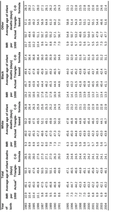
The results of our calculations using the “triangle-based” approximation formula in all years and for all groups are a little bit higher than the exact values calculated from the microdata. There appears to be a systematic difference averaging 2.5 days for the whole population, as well as for Whites and Blacks separately. This can be explained by departures from the conditions required for accuracy, including, for example, that the distribution of births during the year of birth is not uniform (Figure 2). The number of births during the second half of the each year is on average 6% greater than the number in the first half-year. For this reason the number of person-years lived in the upper Lexis triangle is on average 1.4% greater than the corresponding number in the lower triangle. This increases the weight of the upper triangle and leads to overstatement of average age of death in infancy. Note that the differences are almost the same for the whole population, both races, both sexes combined, and for male and female infants separately. However, we consider an error of 2.5 days, or less than 0.7% of a year, to be acceptable.
35 40 45 50
0 5 10 15 20 25
Infant mortality rate (per 1000)
a
0
(
day
s
) Black
White
1983 1983
Table 2: Infant mortality rates (IMRs) and three estimates of the average age of infant deaths in the birth cohorts of 1983–1991 and
1995–2004, by race of mother in the USA
Y ear o f b irt h Tot a l W hi te B lack O the r
IMR pe
r 1000 A v er ag e ag e o f i n fan t d ea th s (d ay s)
IMR pe
r 1000 A v er ag e ag e o f i n fan t d eat h s ( d ay s)
IMR pe
r 1000 A v er ag e ag e o f i n fan t d eat h s ( d ay s)
IMR pe
Figure 2: Average daily number of births by month as a percentage of the annual average daily number births in 1983–1991, 1995–2004, in the USA
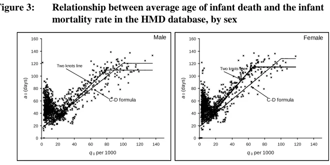
We computed 1a0 from the HMD input data files by the triangle-based formula and the results of each calculation are plotted as “×” markers in Figure 3. Simultaneously, we calculated the average age of infant death using the C-D formula. The thin black line corresponds to these 1a0 estimates. The second heavy line in Figure 3 is our alternative to the C-D formula, described later.
The estimates from the C-D formula tend to be lower than the triangle-based values for 79% of male cohorts and 90% of female cohorts. If we look only at cohorts with 1
q
0<10 per 1000, then the C-D formulas underestimate 1a0 for 98% of our observations. In the example for the USA, 1a0 estimated with the triangle-based formula is on average 2.5 days greater than the actual values calculated from the linked birth and death records. Perhaps analogous circumstances account for the bias in relation to estimates from the C-D formulas. The difference between 1a0 estimated with the C-D formula and that based on the Lexis triangle formula is more than 5 days in 71% of the male and 80% of the female cohorts. If 1q0<10 per 1000, then the difference between 1a0 estimated with the C-D formula and on the basis of the Lexis triangle formula is more than 5 days in 98% of the male and 95% of the female cohorts, and this difference exceeds 10 days in 92% and 89% of male and female cohorts respectively. Detailed analysis of each of the 24 countries listed above (not presented here) has shown that in all countries, secular decrease in 1a0 stopped or slowed down85 90 95 100 105 110
1 2 3 4 5 6 7 8 9 10 11 12
Month
P
er
cen
greatly between the 1960s and 1980s. In one of the countries it was characterized by stagnation and in all the others the trend reversed itself and a0rose. A slow decline in
0
1a synchronous with a decline in the IMR is observed only in the Netherlands and
Slovenia. Unfortunately, data by Lexis triangles for the Netherlands are available only for the cohorts born in the years 1979–1998. The average IMR for male infants in the cohorts born in 1995–1998 is 5.9 per 1000 and average1a0 is 40 days, as opposed to 24.7 days according to the C-D formulas. Major fluctuations in 1a0 in Slovenia complicate our analysis. However, 1a0is on average 33.8 days in the1999–2008 male birth cohorts and 1q0is 4 per 1000, which by the C-D formulas corresponds to 1a0= 22.7 days.
Figure 3: Relationship between average age of infant death and the infant
mortality rate in the HMD database, by sex
Note: Parameters of the two knots lines are presented in Table 3.
Figure 3 also shows that the relationship between 1a0 and the infant mortality rate is complex and the data are noisy, making it difficult to find a simple functional relation of 1a0 from the infant mortality rate by methods such as regression. If the probability of death is less than 10 per 1000, then the Pearson correlation coefficient between infant mortality rates and average ages of observed cohort deaths in infancy is less than 0.03 in magnitude. However, it is possible to find some average relation between these variables that can be used where other information concerning the average age of infant death is unavailable.
Taking Coale and Demeny as a precedent, we looked for a piecewise linear function that best approximates the empirical data, but, in contrast to the former
0 20 40 60 80 100 120 140 160
0 20 40 60 80 100 120 140
q0 per 1000
a
0
(
day
s
)
Male
C-D formula
Two knots line
0 20 40 60 80 100 120 140 160
0 20 40 60 80 100 120 140
q0 per 1000
a
0
(
day
s
)
Female
C-D formula
authors, we sought 3-segment piecewise linear splines on criteria of best fit. We fit the splines using the R routine curfit.free.knot in package Dierckxspline (Doray-Raj and Graves 2009). The package is an extension of the fitting procedures developed by Paul Dierckx and incorporated in the FITPACK package of FORTRAN subprograms (Dierckx 1987). The fundamental nonlinear least squares algorithm is described in Dierckx (1993). The resultant fitted linear splines for males and females are presented in Figure 4.
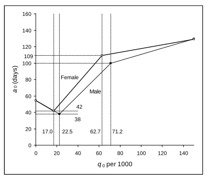
Figure 4: Three-segment piecewise linear spline relating 1a to 0 1q fit to the 0
HMD database, by sex
It is important to note that although the calculations for males and females were performed independently, the abscissas of the left internal knots for males and females agree well with each other: the average female IMR in countries with male IMRs in the interval 22–23 is 17.3 per 1000. This does not hold for the right knots: the male IMR in the interval 70–73 per 1000 corresponds to female IMRs in the interval 52–61, averaging 57 per 1000. As to the rightmost segment, it is clear that 1a0 cannot increase indefinitely with increasing IMR. We assume, as did Coale and Demeny, that at some high level of IMR, 1a0 is constant: in other words the third segment should be a flat line. Unfortunately, there seem to be too few observations in our dataset to estimate the appropriate third knot and the corresponding horizontal segment: our HMD-based dataset includes only 83 observations with male IMRs of more than 71 and 57
0 20 40 60 80 100 120 140 160
0 20 40 60 80 100 120 140
q0 per 1000
a
0
(
day
s
)
Male Female
22.5
17.0 62.7 71.2
observations with female IMRs of more than 64 per 1000. There are only 21 observations of male IMRs and 8 of female IMRs at levels of more than 100 per thousand. In our opinion, these data are not enough for substantively reliable definition of one more knot. Therefore we adopted a 2-step procedure to cover the entire range of
0
1q values. In the first step we estimated a 2-segment piecewise linear approximation
for 1a0 if 1q0< 71 for males and 1q0< 63 per 1000 for females using the curfit.free.knot procedure constrained to a single interior knot. In the second step we continued the 2-segment piecewise line with a horizontal segment that best approximates the leftover points (Figure 3, Table 3). We cannot display a very good fit to the empirical data. Nevertheless, exactly half of the empirical observations are situated above our line.
We offer these formulas as an alternative to the Coale-Demeny equations, for use in circumstances where more direct calculation of 1a0 is not a viable option due to lack of reliable data or for other reasons. Practical recommendations for calculation of the average age at death in infancy based on the central death rate at age 0 are presented in Appendix 3.
Table 3: Parameters of 3-segment piecewise linear splines recommended for
estimation of average age of death in infancy based on the infant mortality rate 1q 0
Lower limits 1q0 Upper limits1q0 Equation
Male
0 0.0226 0.1493 - 2.0367·
0 1q
0.0226 0.0785 0.0244 + 3.4994·
0 1q
0.0785 + 0.2991
Female
0 0.0170 0.1490 - 2.0867·
0 1q
0.0170 0.0658 0.0438 + 4.1075·
0 1q
0.0658 + 0.3141
the C-D formulas, the two-knot line separates the dataset into two almost equal parts: 51.1% of observations for males and 50.4% for females lie above the line.
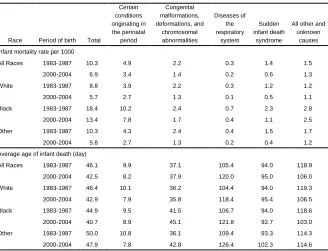
The last results we present pertain to changes in average age of infant death by cause of death. For four racial categories we present results for the first four and last four available cohorts in the US NCHS data, namely the 1983–87 and 2000–04 birth cohorts (Table 4).
Across these periods the infant mortality rate declined from by 6 to by 10 points per thousand. The main contributions to this decline (70%–76%) came from two groups of cause of death: 1) certain conditions originating in the perinatal period and congenital malformations, and 2) deformations and chromosomal abnormalities.
Changes in average age were of lesser magnitude, but it declined for all race categories by some 2–4 days (Table 4).
Table 4: Infant mortality rate and average age of infant death by race of
mother and major causes of death in infancy in the birth cohorts of
1983−1987 and 2000−2004, USA
Race Period of birth Total
Certain conditions originating in the perinatal period
Congenital malformations, deformations, and
chromosomal abnormalities
Diseases of the respiratory
system
Sudden infant death
syndrome
All other and unknown
causes Infant mortality rate per 1000
All Races 1983-1987 10.3 4.9 2.2 0.3 1.4 1.5
2000-2004 6.9 3.4 1.4 0.2 0.6 1.3
White 1983-1987 8.8 3.9 2.2 0.3 1.2 1.2
2000-2004 5.7 2.7 1.3 0.1 0.5 1.1
Black 1983-1987 18.4 10.2 2.4 0.7 2.3 2.8 2000-2004 13.4 7.8 1.7 0.4 1.1 2.5
Other 1983-1987 10.3 4.3 2.4 0.4 1.5 1.7
2000-2004 5.8 2.7 1.3 0.2 0.4 1.2
Average age of infant death (day)
4. Discussion
Using direct observations on age at death in infancy for the USA, and for other countries an approximate formula for calculation of average age of death in infancy verified against the US data, we showed that in the process of infant mortality decline, the negative relationship between the probability of death and the average age at death in infancy disappears after infant mortality reaches some low level. How does this relate to our ideas about the long-term evolution of infant mortality?
In the early 1950s, the eminent French demographer Jean Bourgeois-Pichat created a model of infant mortality that explained why infant mortality decline leads to concentration of infant deaths in the neonatal period (1951a,b). He maintained that there are two types of infant mortality: exogenous mortality due to the influence of postnatal conditions as infants become exposed to the external environment, and endogenous mortality due to conditions of the prenatal period, including congenital diseases. Endogenous mortality is concentrated in the first month of life and its level is relatively stable through time. In general, historical mortality decline has been connected with declining exogenous mortality, including in infancy. Thus, rapid infant mortality decline was observed at ages 1–11 months. Bourgeois-Pichat (1951b) included under the heading of “endogenous mortality” the following four major causes of (infant) death: “congenital defects, prematurity, congenital anomalies, and diseases of earliest childhood”. These categories coincide with the two first items on our list of causes of death in infancy. These two groups alone account for the recent infant mortality decline in low mortality countries, starting from the 1970s. It seems that at present we are witnessing a new stage of mortality decline in the USA, which is largely the result of endogenous mortality decline, in Bourgeois-Pichat’s terminology. The impact of exogenous mortality is smaller. The rapid decline of the endogenous component is what leads to the rise in the average age of infant deaths in the US.
Japan 0 1 2 3 4 5 6
1980 1983 1986 1989 1992 1995 1998 2001 2004 2007
Year P ro b ab il it y o f d eat h ( p er 1000) 0 10 20 30 40 50 60 70 80 90 A ver ag e ag e ( d ays) Average age "Endogenous" "Exogenous" France 0 1 2 3 4 5 6
1980 1983 1986 1989 1992 1995 1998 2001 2004 2007
Year P ro b ab il it y o f d eat h ( p er 1000) 0 10 20 30 40 50 60 70 80 90 A ver ag e ag e ( d ays) Average age "Endogenous" "Exogenous"
Table 5: Infant mortality rates from endogenous and exogenous causes and
average ages of infant deaths by race of mother in the birth cohorts of 1983-1987 and 2000-2004, USA
Infant mortality rate Average age of infant death
Total Endogenous Exogenous Total Endogenous Exogenous
All Races 1983-1987 10.3 7.1 3.2 46.1 18.3 106.7
2000-2004 6.9 4.8 2.1 42.5 16.9 104.2
White 1983-1987 8.8 6.1 2.7 46.4 19.5 106.4
2000-2004 5.7 4.0 1.7 42.9 17.0 103.9
Black 1983-1987 18.4 12.6 5.8 44.9 15.6 107.4
2000-2004 13.4 9.5 4.0 40.7 15.4 102.0
Other 1983-1987 10.3 6.7 3.6 50.0 19.9 105.0
2000-2004 5.8 4.0 1.8 47.9 19.2 113.2
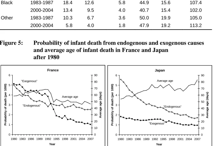
Figure 5: Probability of infant death from endogenous and exogenous causes
and average age of infant death in France and Japan after 1980
The infant mortality rate in Japan in 1988 was about the same as in France in 1995, but the probability of death from exogenous causes was lower than in France by 0.6 per 1000, and the average age in France was lower by 11 days.
Thus, in the mid-1970s, the decline of infant mortality from causes that Bourgeois-Pichat referred to as endogenous, and which in the 1960s seemed unassailable, commenced. In some populations it occurred even more rapidly than the decline of exogenous mortality. This fact explains the observed abatement and even disappearance of the connection between the level and average age of infant mortality. Starting from the 1980s, the average age of infant death became almost independent of the infant mortality rate. However, on average in countries with 1q0 less than 0.017, further decrease of infant mortality is associated with increase in the average age of death in infancy. Our analysis suggests that this is due to the influence of the decline in mortality from endogenous causes of death, which tends to raise the average age of death in infancy.
5. Conclusion
The Coale-Demeny model life tables and the formulas which underlie them have proven to be exceptionally resilient, remaining in use in demographic analysis for three to four decades. Throughout this timespan, the formulas relating 1a0 (k0in their notation) to 1q0 have remained unchanged. This is most remarkable. Ansley Coale and Paul Demeny had 326 life tables, of which 212 pertained to the period prior to 1945 (1966:(7)), and practically all of the rest to the period 1945-1960. According to Coale and Guang (1989), there were hardly any data after 1960 in their collection. In this time period the minimum infant mortality rate for both sexes was more than 12 per 1000. It would be miraculous if the empirical formulas based on this dataset remained accurate up to the present time.
Our assembled data demonstrate that the Coale-Demeny formulas for estimation of the average age of infant death no longer hold for countries with low infant mortality by current standards. In most of these countries, starting from some moment in the process of infant mortality decline, the decrease in the average age of death in infancy has given way to increase. However, the relation between these two indicators is characterized by a reversal in direction, as well as considerable uncertainty, making it difficult to describe with a ‘traditional’ parametric mathematical model. Our two-knot spline is preferable for mortality modeling.
triangle-based formula when not. If estimates of 1a0 are needed and no other data are available other than infant mortality rates by sex, our formulas may be employed. Our analysis shows that these approaches are preferable to the Coale-Demeny formulas at low levels of mortality.
6. Acknowledgements
References
Anderson, R.N., Mininio, A.M., Hoyert, D.L., and Rosenberg H.M. (2001). Comparability of Cause of Death Between ICD-9 and ICD-10: Preliminary Estimates. National Vital Statistics Reports 49(2).
Arias, E., Rostron, B.L., and Tejada-Vera, B. (2010). United States Life Tables, 2005. National Vital Statistics Reports 58(10).
Arriaga, E., Anderson, P., and Heligman, L. (1976). Computer programs for demographic analysis. Washington: United States, Bureau of the Census. Bourgeois-Pichat, J. (1951a). La mesure de la mortalité infantile. Principes et méthodes.
Population 2: 233–248. doi:10.2307/1524151.
Bourgeois-Pichat J. (1951b). La mesure de la mortalité infantile: II. Les causes de décès. Population 6(3): 459–480. doi:10.2307/1523958.
Canudas-Romo, V., Danzhen Y., Yun-Hsiang H., and Tsung-Hsueh L. (2012). About mortality data for Taiwan. The Human Mortality Database. Background and
documentation. http://www.mortality.org/hmd/TWN/
InputDB/TWNcom.pdf.
Chiang, C.L. (1978). The Life Table and Mortality Analysis. Geneva: World Health Organization.
Coale, A. and Guang, G. (1989). Revised regional model life tables at very low levels of mortality. Population Index 55(4): 613–643. doi:10.2307/3644567.
Coale, A.J. and Demeny P. (1966). Regional Model Life Tables and Stable Populations. New York: Academic Press.
Dierckx, P. (1993). Curve and Surface Fitting with Splines. New York: Oxford University Press.
Dierckx, P. (1987). FITPACK user guide Part 1: curve fitting routines. TW report 89. Leuven, Belgium: Katholieke Universiteit, Department of Computer Science. Doray-Raj, S. and Graves, S. (2009). Dierckx Spline: R Companion to “Curve and
Surface Fitting with Splines”. R package version 1.1-4 [http://CRAN.R-project.org/package=DierckxSpline].
Glei, D., Meslé, F., Vallin, J., Wilmoth, J., and Barbieris, M. (2014). About mortality data for France, total population. The Human Mortality Database. Background and documentation. http://www.mortality.org/hmd/FRA /InputDB/FRAcom.pdf.
Jasilionis, D. (2011). About mortality data for the Netherlands. The Human Mortality
Database. Background and documentation. http://www.mortality.org/hmd/NLD/InputDB/NLDcom.pdf.
Jasilionis, D. (2013). About mortality data for the Estonia. The Human Mortality
Database. Background and documentation. http://www.mortality.org/hmd/EST/InputDB/ESTcom.pdf.
Keyfitz, N. and Flieger, W. (1971). Population: facts and methods of Demography. W.H. Freeman.
Mészáros, J. and Jasilionis, D. (2011). About mortality data for the Slovak Republic. The Human Mortality Database. Background and documentation. http://www.mortality.org/hmd/SVK/InputDB/SVKcom.pdf.
MORTPAK (1988). The United Nations Software Package for Mortality Measurement. Batch-oriented Software for the Main frame Computer (ST/ESA/SER.R/78). Non-sales publication.
Philipov, D. and Jasilionis, D. (2012). About mortality data for Bulgaria. The Human Mortality Database. Background and documentation. http://www.mortality.org/hmd/BGR/InputDB/BGRcom.pdf.
Preston, S.H., Heuveline, P., and Guillot, M. (2001). Demography: Measuring and Modeling Population Processes. United States, Malden, Massachusetts: Blackwell Publishing.
Pyrozhkov, S., Foygt, N., and Jdanov, D. (2011). About mortality data for Ukraine. The Human Mortality Database. Background and documentation. http://www.mortality.org/hmd/UKR/InputDB/UKRcom.pdf.
Rychtarikova, J., Jasilionis D., and Grigoriev, P. (2012). About mortality data for the Czech Republic. The Human Mortality Database. Background and documentation. http://www.mortality.org/hmd/CZE/InputDB/CZEcom.pdf. Scholz, R., Jdanov, D., and Kibele, E. (2013). About mortality data for East Germany.
Appendix 1: Proof of the triangle-based formula for average age of
deaths
Consider an annual birth cohort born in year
Y
= [t0,t0+1) that satisfies the following two conditions:– the distribution of births is uniform within
Y
, (the density function of the birth distribution, β(t), is constant withinY
);– the cohort survival function l(x,t), t∈[t0,t0+1) does not depend on date of birth within the age interval [x0,x0+1).
Then the average number of years lived within the age interval [x0,x0+1) among people dying at that agea(x0) is equal to the share of the number of deaths in the upper Lexis triangle in the total number of deaths at agex0.
Proof. Let bY denote the initial size of the birth cohort, and let lYx stand for the cohort survival function. It is obvious that Y
t
t
b dt
t =
∫
+10 0
) (
β and l(x,t)=lY(x)for
) 1 , [0 0+
∈ t t
t . It follows that the number of cohort members attaining age x0 by the end of calendar year t0 is equal to
Y x Y
L b
0
1
⋅ , where =
∫
+1
0 0 1L0 l (x
θ
)dθ
Y Y
x represents the
cumulated survivorship function corresponding to lY(x)in the age interval x0 to x0+1. In general, this number of people is
∫
+ ⋅ − + +1
0
0
0 ) ( 1, )
(
θ
θ
θ
θ
β
t l x to d . Taking intoaccount the properties of the cohort assumed above, this number of people is equal to
. )
( )
1
( 1 0
1
0 0 1
0 0
Y x Y Y
Y Y
Y
L b d x l b d x
l
b
∫
−θ
+θ
= ⋅∫
+ξ
ξ
= ⋅Let the parallelogram ABCD (Figure 1-1)correspond to the cohort and age interval under consideration. We should prove that the number of deaths in the triangle BCD divided by the total number of deaths in the parallelogram ABCD is Y
x
a 0
Figure 1-1: Lexis parallelogram of deaths in a birth cohort
The number of survivors at age x0 is equal to Y x Y
l b
0
⋅ (the segment AB) and at age
1
0+
x is equal to bY lYx 1 0+
⋅ (the segment DC). The segment BD corresponds to the
number of survivors to the end of calendar years Y+x0and is equal to V x Y L
b 0
1
⋅ .Thus the
number of deaths in the upper triangle, BCD, is (1 1) 0 0 V x V x Y l L
b ⋅ − + . If we replace LVx 0
1
with the formula for its calculation 1 1 1 ( 1) 0 0 0 0 0 Y x Y x Y x Y x Y
x l a l l
L = + + ⋅ − + we find that the
number of deaths in the upper triangle is 1 ( 1) 0 0 0 Y x Y x Y Y
x b l l
a ⋅ ⋅ − + . The product
) ( 1 0 0 Y x Y x Y l l
b ⋅ − + is exactly the number of deaths in the parallelogram ABCD. So, the ratio
of BCD to ABCD is Yx
Appendix 2: Possible influence of the transition to ICD-10 on
indicators of infant mortality by cause of death
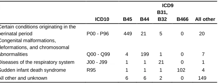
Prior to the implementation of ICD-10, the US NCHS conducted a comparison study in which a sample of death records filed in 1996 was coded according to both the ICD-9 and ICD-10 classifications. From the cross tabulation of deaths by cause according to the two respective classifications, “comparability ratios” were calculated (Anderson et al. 2001), each indicating the ratio of deaths in an aggregated cause category coded under the ICD-10 rules to the number of deaths in the same category coded under the ICD-9 rules. These cross-classifications can also be used to develop “transition coefficients” for converting underlying causes of death from ICD-9 categories into ICD-10 equivalents. We have opted not to employ these in our analysis, and have instead aggregated the deaths by detailed cause under the classification in effect in the respective years into a small number of broad groups of cause of death.
In our analysis we employed 4 broad categories of cause of death, plus a residual category of “all other causes”. These broad categories were not developed initially from either the ICD-9 or the ICD-10 classifications, although both classifications were mapped at the 4-digit level into the 5 broad categories. Table 2-1 presents a cross tabulation of infant deaths coded on both the ICD-9 and ICD-10 classification from the NCHS comparison study conducted in 1996. The detailed causes of death for each of the two ICD versions have been grouped into the 5 broad categories used in the present analysis. Only infant deaths that were assigned valid codes under both 9 and ICD-10 have been tabulated. The bivariate data are presented as deaths per thousand live births.
Table 2-1: Correspondence between deaths classified according to ICD-9 and ICD-10 classifications of causes of death, USA (per 1000)
ICD10
ICD9
B45 B44 B31,
B32 B466 All other
Certain conditions originating in the
perinatal period P00 - P96 449 21 5 0 20
Congenital malformations, deformations, and chromosomal
abnormalities Q00 - Q99 4 199 1 0 7
Diseases of the respiratory system J00 - J99 1 1 21 0 1
Sudden infant death syndrome R95 1 1 1 102 4
All other and unknown 6 6 2 0 149
Note: Only record axis codes are considered. Causes of death for which there was no occurrence in 1996 are not represented, for obvious reasons. This tabulation refers to all infant deaths that could be coded by both ICD-9 and ICD-10, which are less than the number of infant deaths registered in 1996.
Appendix 3: Practical recommendations for calculation of the
average age at death in infancy
1a0based on the central death rate
0
1M
at age 0.
The equations for 1a0 are 3-segment piecewise linear splines on1q0. At each 1q0 -segment 1a0 is a linear function of 1q0. In terms of 1M0, the average age is a relatively exotic function that can be derived from the two simultaneous equations
0 1 0 1
0 1 0
1
0 1 0
1
) 1 (
1 a M
M q
q B A a
⋅ − + =
+ =
.
This function is the solution of the quadratic equations in1a0 whose coefficients are linear functions of 1M0. However, the function that describes dependency 1a0 from
0
1q is an approximate empirical function. Therefore excessive precision is unnecessary
Table 3-2: Parameters of 3-segment piecewise linear splines recommended for estimation of average age of death in infancy based on the central
death rate 1M 0
Lower limits 1M0 Upper limits1M0 Equation
Male
0 0.02300 0.14929-1.99545∙1M0
0.02300 0.08307 0.02832+3.26021∙1M0
0.08307 + 0.29915
Female
0 0.01724 0.14903-2.05527∙
0 1M
0.01724 0.06891 0.04667+3.88089∙
0.06891 + 0.31411
We offer these formulas for use in circumstances where only 1M0is available.