OF COMPACT OPERATORS
by James Ford
A thesis
submitted in partial fulfillment of the requirements for the degree of
Master of Science in Mathematics Boise State University
DEFENSE COMMITTEE AND FINAL READING APPROVALS
of the thesis submitted by
James Ford
Thesis Title: Joint Inversion of Compact Operators Date of Final Oral Examination: 24 May 2017
The following individuals read and discussed the thesis submitted by student James Ford, and they evaluated his presentation and response to questions during the final oral examination. They found that the student passed the final oral examination. Jodi Mead, Ph.D. Chair, Supervisory Committee
John Bradford, Ph.D. Member, Supervisory Committee Grady Wright, Ph.D. Member, Supervisory Committee
First, I would like to thank my advisor Dr. Jodi Mead, who introduced me to inverse problems and academic research. Her patience and insights throughout my time at Boise State University have been invaluable. I would also like to extend my gratitude to the other members of my thesis committee, Dr. Grady Wright and Dr. John Bradford. All of them have been continually encouraging and are exemplary researchers whose work I try to model my own after.
My sincere thanks goes out to the Department of Mathematics whose financial support has allowed me to attend a number of impactful conferences and workshops during my time as a student. I also thank my fellow classmates in the mathematics program. Enduring this experience together made it more productive and vastly more enjoyable.
I thank my family: My parents Ann and Chris, who fostered my intellectual curiosity from a young age and have always supported my decisions; and my brother Ben, whose relentless competition has continuously pushed me to become better.
Finally, I wish to thank Cass, whose impact on my life is immeasurable. Her unending support has made all of this possible.
The first mention of joint inversion came in [22], where the authors used the singular value decomposition to determine the degree of ill-conditioning in inverse problems. The authors demonstrated in several examples that combining two models in a joint inversion, and effectively stacking discrete linear models, improved the conditioning of the problem. This thesis extends the notion of using the singular value decomposition to determine the conditioning of discrete joint inversion to using the singular value expansion to determine the well-posedness of joint linear operators. We focus on compact linear operators related to geophysical, electromagnetic subsurface imaging.
The operators are based on combining Green’s function solutions to differential equations representing different types of data. Joint operators are formed by extend-ing the concept of stackextend-ing matrices to one of combinextend-ing operators. We propose that the effectiveness of joint inversion can be evaluated by comparing the decay rate of the singular values of the joint operator to those from the individual operators. The joint singular values are approximated by an extension of the Galerkin method given in [9, 18]. The approach is illustrated on a one-dimensional ordinary differential equation where slight improvement is observed when naively combining differential equations. Since this approach relies primarily on the differential equations representing data, it provides a mathematical framework for determining the effectiveness of joint inversion methods. It can be extended to more realistic differential equations in order to better inform the design of field experiments.
ABSTRACT . . . vi
LIST OF FIGURES . . . ix
1 Introduction . . . 1
2 Inversion . . . 4
2.1 Discrete inversion . . . 4
2.1.1 Linear problems . . . 5
2.1.2 Singular value decomposition . . . 5
2.1.3 Conditioning and Regularization . . . 8
2.2 Inversion with compact operators . . . 10
2.2.1 Green’s functions . . . 10
2.2.2 Singular value expansion . . . 12
2.2.3 Conditioning and ill-posedness . . . 14
2.2.4 Regularization . . . 18
3 Joint Inversion . . . 23
3.1 Discrete joint inversion . . . 23
3.1.1 Linear problems . . . 23
3.1.2 Green’s functions example . . . 24
3.2 Joint inversion with compact operators . . . 26
3.2.2 Singular values . . . 28
3.2.3 Approximation of SVE with SVD . . . 32
4 Application with compact operators . . . 37
4.1 Individual operators . . . 37
4.2 Joint operator . . . 41
4.3 Joint singular values . . . 44
5 Conclusions and future work . . . 48
REFERENCES . . . 50
1.1 Electrical resistivity setup [4] (left) and ground penetrating radar [5] (right) . . . 1
2.1 Singular values of A on a semi-log scale (a), and a log-log scale (b) . . . . 18
3.1 Singular values of individual operators and joint operator . . . 26 3.2 Parametric curve defined by C(coskx) fork ∈[−5,5] . . . 29
4.1 Singular values of individual operators . . . 42 4.2 Analytical singular values and Galerkin method approximations using
orthonormal box functions . . . 45 4.3 Approximate singular values of the joint operatorCon a semi-log scale
(a), and a log-log scale (b) . . . 46 4.4 Approximate singular values of the individual operatorsA andB, and
the joint operator C on a semi-log scale (a), and a log-log scale (b) . . . 47
CHAPTER 1
INTRODUCTION
This thesis is motivated by electromagnetic imaging of the Earth’s subsurface using two data collection methods – ground penetrating radar (GPR) and electrical resistivity (ER), both depicted in Figure 1.1. The ER survey on the left uses electrodes to introduce and measure current within the Earth’s subsurface, from which the electrical conductivity can be estimated within a localized region. The GPR survey on the right involves a transmitter emitting radar pulses into the subsurface. The energy reflected back by dielectric interfaces within the subsurface is recorded by the receiver, and conductivity can also be inferred. Joint inversion of these data can give conductivity estimates on a vast range of frequency bands from 100 to 109 Hz. A
comprehensive introduction to geophysical electromagnetic imaging can be found in [19, 23].
Maxwell’s equations govern the behavior of both ER and GPR, relating input sources to observable responses [14]. If we assume the domain we are interested in imaging is linear and isotropic, Maxwell’s equations can be decoupled into the wave equation and the diffusion equation. Under these assumptions, the damped wave equation governs GPR:
ε∂
2E
∂t2 +σ
∂E ∂t =
1 µ∇
2E +f,
where E is the electric field component, f is the source; while the parameters µ, ε, andσ are scalar functions of space representing magnetic permeability, dielectric per-mittivity and conductivity, respectively. The forward problem takes the parameters as input and produces the electric field as a function of space and time. The inverse problem takes discrete measurements of the electric field and produces parameter estimates that can be used to image the Earth’s subsurface.
Alternatively, the diffusion equation governs ER and assumes no time dependence of the electric field:
−∇ ·σ∇φ =∇ ·Js,
where Js is the source current density and φ is the electric field potential. Similar to GPR, given discrete measurements of the electric field potential, the conductivity can be estimated through an inversion.
these conditions arise with great frequency in many areas of science and engineer-ing, including electromagnetic subsurface imaging [11]. Since inverse problems are notoriously ill-posed, approaches to solving them will be the focus of this thesis.
The primary tools we will use for the analysis of inverse problems are the singular value decomposition (SVD) and its continuous analogue, the singular value expansion (SVE). We begin in Chapter 2 with a brief introduction to the solutions of discrete inverse problems using the SVD. Green’s functions are then introduced since they continuously describe the solution of differential equations as a function of unknown parameters or sources. The corresponding operators are consequently decomposed using the SVE. A simple example is given with the focus on the behaviors of the corresponding singular values. Tikhonov regularization in the context of the SVE is also described.
CHAPTER 2
INVERSION
2.1
Discrete inversion
Data collection is typically represented as a finite number of measurements taken at discrete points in space and time. It is therefore natural to first consider a discrete inverse problem, with observations denotedb= (b1, b2, . . . bm) and parameters we seek to recover denoted x= (x1, x2, . . . xn). Then, with g being the model relating x and b, we attempt to solve the system g(x) = b, or
g1(x1, x2,. . . , xn) g2(x1, x2,. . . , xn)
.. .
gm(x1, x2,. . . , xn)
= b1 b2 .. . bm
for the parameter vectorx. As previously mentioned, such problems may be ill-posed. A careful analysis of the modelg can reveal if the problem has any solutions, a unique solution and if it is stable. Such insights can inform methods that allow us to proceed in any case.
problems as well as the methods used to analyze and solve them. This background will set the stage for the continuous analogues developed in this thesis.
2.1.1 Linear problems
The simplest case of discrete inverse problems occurs when the model and param-eters are related linearly. That is,
g1(x1, x2,. . . , xn) g2(x1, x2,. . . , xn)
.. .
gm(x1, x2,. . . , xn)
=
a11x1+a12x2+· · ·+a1nxn a21x1+a22x2+· · ·+a2nxn
.. .
am1x1+am2x2+· · ·+amnxn
In this case, the model can be represented as matrix, and we solve Ax=b to recover the parameters. We will devote our attention to linear problems. The assumption of linearity is not so restrictive, since most non-linear methods involve iteratively solving a linear problem. Therefore this thesis is devoted to analyzing and solving linear problems.
2.1.2 Singular value decomposition
The primary tool used for the analysis of linear inverse problems is the singular value decomposition (SVD). This algebraic decomposition represents a special case of the singular value expansion (SVE), which will be discussed in 2.2.2.
Theorem 2.1.1 (Singular Value Decomposition). Let A ∈ Rm×n be a matrix of rank r. Then, there exist orthogonal matrices U ∈Rm×m and V ∈
A=UΣVT, Σ =
Σr 0 0 0
,
where Σ∈Rm×n, Σ
r = diag(σ1, σ2, . . . σr) and
σ1 ≥σ2 ≥. . . σr >0.
Letting vj and uj be the jth columns of V and U respectively, we have that
Avj =σjuj, ATuj =σjvj, for j = 1, . . . , n ATuj = 0, for j =n+ 1, . . . , m
Proof. See [15].
This decomposition is enormously useful. For example, the norm of a vector is invariant under multiplication by an orthogonal matrix. So when considering Ax = UΣVTx, the scaling affect of the model can be isolated to Σ. This allows us to classify if solutions will exist and the conditioning of the model. Additionally, this can yield insights into the importance of each parameter, xi. Parameters associated with large singular values will have a significantly greater influence on the outcome of the forward problem and can therefore be classified as more important [22].
In the case of a square matrix with full rank, r = m = n, we can very easily formulate the inverse ofA using the SVD, and therefore the solution to Ax=b:
A−1 =VΣ−1UT, x=VΣ−1UTb.
the inverse does not exist. In the case of full rank, overdetermined systems we can find the least squares solution to the problem; that is, the parameter vector that minimizes
||b−Ax||2 2.
The solution estimate in this case is
ˆ
x= ATA−1ATb.
The generalized inverse allows us to define the solution estimate in terms of the SVD when A is not invertible. We construct the generalized inverse by first defining Σ†∈Rn×m as
Σ†=
Σ−1
r 0 0 0
.
Then we can define the generalized inverse A† as
A†=VΣ†UT.
Further, we can define a generalized (or pseudo) inverse solution x† by
x†=A†b
=VӆUTb =
r
X
i=1
uTib σi
vi.
2.1.3 Conditioning and Regularization
As stated previously, the third property that a well-posed problem should pos-sess is stability, i.e., the solutions behavior changes continuously with the initial conditions. Typically, discrete problems are solved computationally. Therefore, the property we are interested in becomes numerical stability or conditioning. Given the SVD of a model, we are able to determine to what degree the inverse solution will be affected by perturbations in the inputs. The metric by which ill-conditioning is measured is called the condition number.
Definition 2.1.1. (Condition number) The condition number of A is defined to be κ(A) = σ1/σr, where r=rank(A).
As can be seen above, the generalized solution, x†, is dependent on the inverse
of the singular values of A. If σ−11 << σ−1
p , for some p where 1 < p ≤ r, then the portion of the summation
r
X
i=p uT
i b σi
vi
will dominate the solution. The ratio of the largest singular value to the smallest quantifies this effect. For κ(A) large, the values in b associated with σr will be scaled by a much greater amount than the values associated with σ1. Therefore,
small perturbations in b can result in large changes to the solution. There are a vast number of regularization methods for addressing this issue of ill-conditioning [1, 11, 10]. We will focus on two in particular, the truncated singular value decomposition and Tikhonov regularization.
Ak =UΣVT, Σ =
Σk 0 0 0
,
where Σk = diag(σ1, σ2, . . . , σk). Then the solution using this truncated matrix is
xk† =A†kb = k X i=1 uT i b σi
vi.
The matrixAkis the best rankkapproximation toA[10]. If we cut off a small number singular values, we will have a very good approximation of the original matrix, and our inverse solution will be less susceptible to perturbations inb. The choice of truncation value is challenging and not within the scope of this thesis. Though, in general, it is advantageous to keep as many singular values as possible, while maintaining stability.
Tikhonov regularization is another method of combating ill-conditioning. Here, we solve a damped least squares problem
min
x ||b−Ax||
2 2+α
2||x||2 2, or equivalently min x b 0 − A αI x 2 2 .
For large enough α, this damped least squares problem always has a solution. The solution xα
†, is dependent on α and can be expressed in terms of the SVD of A [1].
Namely,
xα† = r X i=1 σ2 i σ2
i +α2 uT
i b σi
By writing the solution in this form, we see that the contribution of singular values smaller than alpha are damped out. However, we still have the challenge of choosing an α that improves the conditioning, but does not significantly change the problem. Methods for choosing the regularization parameter include the discrepancy principle, L-curve and generalized cross validation (GCV) [1], but these fall outside the scope of this thesis.
2.2
Inversion with compact operators
In this section, we extend the notions in 2.1 to continuous functions and compact linear operators. Since we are interested in physical phenomena modeled by differen-tial equations, we wish to consider operators with some physical significance. Green’s functions solutions of inhomogeneous differential equations determine the response of the physical system for given a source. The integral operators corresponding to Green’s functions are therefore the compact operators we will investigate. They provide a physically motivated, yet abstract paradigm in which we may consider inverse problems. A thorough discussion of Green’s functions and their applications can be found in [3].
2.2.1 Green’s functions
LetLA=LA(t) be a linear differential operator. Then the corresponding Green’s function, KA(t, s) satisfies
LAKA(t, s) =δ(t−s), (2.1)
(delta function).
Given the Green’s function, we can find the solution to the inhomogeneous equa-tion LAu(t) = f(t) for a given specific, f. This is accomplished by integrating both sides of equation (2.1) againstf(s) over s in the domain Ω,
Z
Ω
LAKA(t, s)f(s)ds=
Z
Ω
δ(t−s)f(s)ds.
Since LA is a an operator acting only on t, it can be moved outside of the integral. Therefore we have,
LA
Z
Ω
KA(t, s)f(s)ds
=f(t).
Thus the solution to LAu(t) = f(t) for a given sourcef is
u(t) =
Z
Ω
KA(t, s)f(s)ds.
In other words, integrating the Green’s function against the source gives the response of the system to that source.
If we define the operator A to be
Ah(t) =
Z
Ω
KA(t, s)h(s)ds,
first work through some general results concerning compact operators.
2.2.2 Singular value expansion
When considering discrete inverse problems, the singular value decomposition is the tool of choice for rigorous analysis of the problem and its least squares solution. The continuous extension of this tool is the singular value expansion (SVE) [6, 9, 16, 17]. When originally developed by Smith, the singular value decomposition of a matrix was treated a special case of the more general singular value expansion. A history of the early development of the SVD/SVE can be found in [20]. Our study of general linear inverse problems will proceed with the singular value expansion as our primary tool. In particular, we will use the SVE for compact operators acting on Hilbert spaces. This is the analogous concept of a matrix acting on a finite dimensional vector space.
Definition 2.2.1. (Compact operator) Let H and HA be Hilbert spaces and let A : H → HA be a linear operator. We say A is compact if the image under A of a bounded subset of H is a precompact subset of HA.
With the assumption of compactness, a significant amount of matrix theory can be extended to continuous operators. In particular, using the SVE we decompose an operator into orthogonal functions as we would decompose a matrix into orthogonal vectors in the SVD.
Note that we do not wish to consider the case where A has only finitely many singular values, nor the case where A is not compact.
{φk} ⊂ H and {ψk} ⊂ HA and positive numbers σ1 ≥ σ2 ≥ · · · converging to zero,
such that
A=
∞
X
k=1
σkψk⊗φk, and A∗ =
∞
X
k=1
σkφk⊗ψk.
We define ψk⊗φk as
(ψk⊗φk)h =hh, φkiHψk,
for allh∈H. Note that A∗ is also a compact linear operator and denotes the adjoint of A. Furthermore,
Aφk =σkψk for all k
and
Ah=
∞
X
k=1
σkhφk, hiHψk for all h∈H.
Additionally, {φk} is a complete orthonormal set for N(A)⊥ and {ψk} is a complete orthonormal set for R(A).
Proof. See [6] or [7].
To derive the singular values analytically, we typically consider solving
A∗Aφ=σ2φ.
This yields a family of singular function, singular value pairs{(σk, φk)}∞k=1. As we will
In section 2.1.2 we defined the discrete generalized inverse for a matrix A that operates on real, finite dimensional Hilbert spaces with A: Rn → Rm. Written as a summation,
A†= r
X
i=1
σ−i 1vi⊗ui = r
X
i=1
viuTi σi
.
The solution that minimizes kAx−bk22 is given by
x†=A†b =
r X i=1 uT i b σi vi.
Now suppose H and HA are infinite dimensional Hilbert spaces, with A : H → HA a compact linear operator having singular system {σi, φi, ψi} as defined in Theorem 2.2.1. The generalized inverse is expressed in an analogous manner,
A† =
∞
X
k=1
σk−1φk⊗ψk. (2.2)
It is clear from this formulation thatA† is not a compact operator, sinceσ−k1 increase in an unbounded manner [13, 16].
As with the discrete case, it will most likely be the case that we cannot solve Ah=f exactly. we again find the least squares solution that minimizeskAh−fk2H
A. In terms of the SVE, this gives,
h=A†f =
∞
X
k=1
σk−1(φk⊗ψk)f =
∞
X
k=1
hψk, fiHA σk
φk for all f ∈D A†
.
2.2.3 Conditioning and ill-posedness
decaying towards zero. The condition number is therefore not a sufficient metric by which to measure ill-posedness. As in the discrete case, it is clear that small singular values (relative toσ1) will disproportionately amplify the contribution from
corresponding singular vectors or functions. If there is noise in the data, this too will be amplified, perhaps to an unacceptable level.
We characterize the ill-posedness of the problem in terms of the decay rate of its singular values. In particular, if σk(A) decays like k−q, we call q the degree of ill-posedness. Thus larger values ofqindicate larger degrees of ill-posedness. In Chapter 3, we will use this metric to determine how joint inversion improves single inversions. Let us consider the following example to illustrate this measure of ill-posedness.
Example
Define the compact linear operator A:H →HA, where H =HA=L2(0,1), by
Ah(t) =
Z t
0
h(s)ds,
Then, the adjoint operator A∗ :HA→H is
A∗f(t) =
Z 1
t
f(s)ds
and the self-adjoint operatorA∗A:H →H is
A∗Ah(t) =
Z 1
t
Z s
0
h(τ)dτ
ds.
A∗Aφ=λφ(t) = Z 1 t Z s 0 φ(τ)dτ ds.
Notice, that substituting in t = 1 to both sides of the integral equation gives us φ(1) = 0 for λ 6= 0. Differentiating both sides of the equation with respect to t and applying a Leibniz integral rule yields
λφ0(t) = d dt Z 1 t Z s 0 φ(τ)dτ ds = Z 1 t ∂ ∂t Z s 0 φ(τ)dτ ds− Z t 0 φ(τ)dτ =− Z t 0 φ(τ)dτ.
Substituting int= 0 to both sides of the above equation gives usφ0(0) = 0 forλ 6= 0. Differentiating both sides of the equation again with respect to t yields
λφ00(t) = −d dt
Z t
0
φ(τ)dτ =−φ(t).
We can now observe that the original problem is equivalent to
λφ00+φ= 0, with φ(1) =φ0(0) = 0.
To find the solution of this boundary value problem, consider the roots of the auxiliary equation λr2+ 1 = 0. They are
r1 =
1i √
λ, r2 = −1i
This gives us the general solution to the ODE and its derivative as
φ(t) = c1cos
t √ λ
+c2sin
t √ λ ,
φ0(t) = −√c1 λsin t √ λ
+ √c2 λcos t √ λ .
Using the boundary conditions φ(1) =φ0(0) = 0, we deduce that
c2 = 0, and
λk =
4 (2k−1)2π2.
Thus the singular functions are of the form
φk(t) =c1cos
2k−1 2 πt,
where c1 must be chosen to satisfy the orthonormality condition hφk, φkiH = 1, for
k = 1,2, . . . ,∞. This yields a family of functions,
φk(t) = √
2 cos2k−1
2 πt, k∈N, and λk =
4
(2k−1)2π2, k∈N.
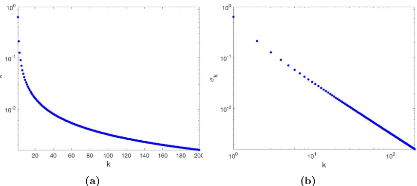
The singular values of the compact operator A are the square roots of λ, that is
σk = 2
(2k−1)π, k ∈N.
(a) (b)
Figure 2.1: Singular values of A on a semi-log scale (a), and a log-log scale (b)
diffusion equation is an example of a severely ill-posed problem.
2.2.4 Regularization
The negative effect decaying singular values have on the parameter estimates in an ill-posed problem can be alleviated with regularization. In infinite dimensional Hilbert spaces, a truncated SVE approximation to the operatorAcan be formed analogously to the truncated SVD of a matrix. This requires the truncation of infinitely many sin-gular values, and we will not investigate this finite sum approximation. Alternatively, we focus on Tikhonov regularization for compact operators.
Tikhonov regularization
to consider the space HA×H ={(hA, h) :hA ∈HA, h∈H} which is a Hilbert space under the inner product
h(hA,1, h1),(hA,2, h2)iHA×H =hhA,1, hA,2iHA +hh1, h2iH.
Now we may define a new operator Tλ :H →HA×H by
Tλh= (Ah, √
λh).
In place of kAh−fk2H
A, we instead consider minimizing
kTλh−(f,0)k2HA×H =kAh−fk
2
HA +λkhk
2
H.
Note thatλ is being used as a regularization parameter, and not an eigenvalue.
Theorem 2.2.2. Supposeλ >0. ThenR(Tλ) is closed andN(Tλ) is trivial. Therefore Tλh = (f,0) has a unique least squares solution for all f ∈HA, [6].
Proof. Consider the normal equation for this problem:
T∗T h=T∗(f,0) T∗(Ah,
√
λh) =T∗(f,0) A∗Ah+λh=A∗f +√λ·0 (A∗A+λI)h=A∗f.
Tikhonov regularization replaces the not necessarily invertible operatorA∗A with the necessarily invertible (A∗A+λI) in the normal equations. A solution is guaranteed for appropriateλ, however we have restricted the space of acceptable solutions.
We now examine the regularized solutions expressed in terms of the singular value expansion of A. Given the singular value expansion of A and its adjoint A∗, A∗A applied to h can be expressed as
A∗Ah=A∗
∞
X
k=1
σkhφk, hiHψk
!
=
∞
X
k=1
σkhφk, hiHA∗ψk
=
∞
X
k=1
σ2khφk, hiHφk.
Equivalently,
A∗A=
∞
X
k=1
σ2kφk⊗φk.
Recall that {φk} is an orthonormal set for the N(A)⊥. So, h ∈ H can be expressed as
h= projN(A)⊥h+ projN(A)h =
∞
X
k=1
hh, φkiHφk+ projN(A)h
(A∗A+λI)h=A∗A
∞
X
k=1
hh, φkiHφk+ projN(A)h
!
+λ
∞
X
k=1
hh, φkiHφk+ projN(A)h
!
=A∗A
∞
X
k=1
hh, φkiHφk
!
+λ
∞
X
k=1
hh, φkiHφk+λprojN(A)h
=
∞
X
k=1
hh, φkiHA∗Aφk+
∞
X
k=1
λhh, φkiHφk+λprojN(A)h
=
∞
X
k=1
σ2khh, φkiHφk+
∞
X
k=1
λhh, φkiHφk+λprojN(A)h
=
∞
X
k=1
σk2+λhh, φkiHφk+λprojN(A)h.
Equivalently,
(A∗A+λI) =
∞
X
k=1
σ2k+λφk⊗φk+λprojN(A).
This allows us to consider solutionsh(λ) ∈Hsatisfying (A∗A+λI)h(λ) =A∗f in terms of the SVE of A. From our above expansions, we can see that h(λ) must equivalently satisfy
∞
X
k=1
σ2k+λhh(λ), φ
kiHφk+λprojN(A)h(λ) =
∞
X
k=1
σkhψk, fiHAφk.
Since the two summations are linear combinations of{φk}, they represent elements in N(A)⊥ . Therefore, it must be the case that λprojN(A)h(λ) = 0, and h(λ) lies in
N(A)⊥. So we have thath(λ) must satisfy
∞
X
k=1
σk2+λhh(λ), φkiHφk =
∞
X
k=1
=⇒ σ2k+λhh(λ), φ
kiH =σkhψk, fiHA for all k∈N =⇒ hh(λ), φ
kiH = σk σ2
k+λ
hψk, fiHA for all k ∈N
=⇒ h(λ)=
∞
X
k=1
σk σ2
k+λ
hψk, fiHAφk.
This implies that the generalized inverse operator for the modified least squares problem is
A†λ = (A∗A+λI)−1A∗ =
∞
X
k=1
σk σ2
k+λ
φk⊗ψk.
Notice that
σk σ2
k+λ
→0, ask → ∞.
Therefore the operator A†λ is bounded, and inverse solutions depend continuously on f.
CHAPTER 3
JOINT INVERSION
3.1
Discrete joint inversion
3.1.1 Linear problems
The earliest mention of joint inversion comes from Vozoff and Jupp in their 1975 paper [22]. Here the authors considered combining several different kinds of geophysical measurements to avoid some of the ambiguity inherent in the individual methods. Mathematically speaking, they looked at a problem of two linear models A and B dependent on the same set of unknown parameters x, with corresponding data d1 and d2 respectively:
Ax=d1 and Bx=d2.
When AandB are ill-conditioned, the individual problems require regularization. Alternatively, Vozoff and Jupp explored the potential of using less regularization by solving the joint inversion problem
A B
x=
d1
d2
To measure the effectiveness of this approach, the authors considered the decay rate of the singular values of A, B, and
A B
. In several examples, they demonstrated
that the singular value decomposition of
A B
yielded a significant increase in the
number of usable values, as compared to A and B individually.
In this thesis we extend the discrete results of Vozoff and Jupp to a continuous setting. In particular, we measure the effectiveness of combining operators in an analogous way; the decay rate of singular values from individual and joint compact operators will be compared.
3.1.2 Green’s functions example
First, we apply the ideas presented by Vozoff and Jupp to a pair of discretized Green’s functions. As motivated by the imaging example in the introduction, we choose the Green’s functions for the wave and diffusion equations in time and one spatial variable.
The Green’s function for the wave and diffusion equations for homogeneous media inx and t are
Kw = 1
2H((t−τ) + (x−ξ))H((t−τ)−(x−ξ)), Kd=pH(t−τ)
4π2(t−τ)exp
−(x−
ξ)2
4(t−τ)
respectively, where H denotes the Heaviside function [3].
u(x, t) =
Z Z
K(x, t, ξ, τ)f(ξ, τ)dξdτ.
Using a two dimensional midpoint quadrature rule, we can approximate our solution on an m×n grid as
u(xi, tj)≈ m
X
l=1
n
X
k=1
K(xi, tj, ξk, τl)f(ξk, τl)∆ξ∆τ.
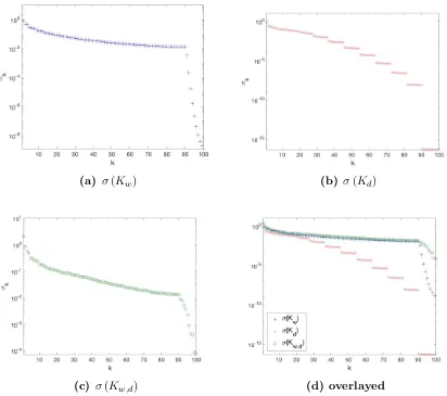
With some simple reshaping, we approximate the operation of double integration againstK as a matrix multiplication so that we solveAf =ufor the source function. The resulting singular values of the matrices from the discretized individual and joint operators are plotted in Figure 3.1. The wave equation in (a) had singular values decay slowly until the ninetieth. Then the singular values rapidly approached zero. The diffusion equation in (b) had singular values that decayed more rapidly than the wave equation, exhibiting noticeable drops every ten values past the forty-fifth, eventually dropping to machine precision. The joint operator in (c) had singular values that tapered off far less dramatically than either the wave or diffusion equation. It is significantly better conditioned than either individual model.
(a) σ(Kw) (b) σ(Kd)
(c) σ(Kw,d) (d) overlayed
Figure 3.1: Singular values of individual operators and joint operator
3.2
Joint inversion with compact operators
3.2.1 Joint operators
As with Tikhonov regularization, our joint operator will map into the Cartesian product of two Hilbert spaces. However, rather than consider the mathematically defined spaceH in Tikhonov regularization, we introduce the new physical spaceHB defined by an additional data collection technique.
Definition 3.2.1. (Hilbert space direct sum) Let HA and HB be Hilbert spaces and
HA⊕HB ={(hA, hB) :hA ∈HA, hB ∈HB}.
Define an inner producth·,·i on HA⊕HB by
h(hA,1, hB,1),(hA,2, hB,2)iHA⊕HB =hhA,1, hA,2iHA +hhB,1, hB,2iHB.
With respect to this inner product, HA⊕HB is a Hilbert Space called the Hilbert space direct sum of HA and HB.
Remark. LetA :H →HA and B :H →HB be compact operators from the Hilbert space H to the Hilbert spaces HAand HB respectively. Define C :H →HA⊕HB as Ch = (Ah, Bh), for all h ∈ H. Then C is a compact operator between two Hilbert spaces, [2]. Therefore, C admits a singular value expansion.
Example
Define the Hilbert spaces H=L2(0,2π), andHA=HB =R. Define the compact operators A:H →HA and B :H →HB as
Ah =
Z 2π
0
h(y)δ(y−5)dy, Bh=
Z 2π
0
h(y)δ(y−7)dy.
DefineC :H →HA⊕HB as
Ch= (Ah, Bh) =
Z 2π
0
h(y)δ(y−5)dy,
Z 2π
0
h(y)δ(y−7)dy
.
Now let us consider the image of a subset ofHunderC. DefineS ={coskx:k∈R, x∈[0,2π]}, a continuum of cosine functions of each possible frequency. So for each frequency
k ∈Rthe mapping of coskx under C is
C(coskx) =
Z 2π
0
cos(ky)δ(y−5)dy,
Z 2π
0
cos(ky)δ(y−7)dy
(3.1)
= (cos(k·5),cos(k·7)). (3.2)
Since the codomain ofC is HA⊕HB =R2, we can represent the image of S underC graphically; see Figure 3.2.
3.2.2 Singular values
The singular values of the joint operator are found by solving C∗Cφ=σ2φ. With
Cdefined as in the remark above,hA∈HAandhB ∈HB, the adjointC∗ :HA⊕HB → H is
Figure 3.2: Parametric curve defined by C(coskx) for k∈[−5,5]
Expanding we get
σ2φ=C∗Cφ =C∗(Aφ, Bφ)
=A∗Aφ+B∗Bφ. (3.3)
Ah =
Z
Ω
Kwh and, Bh=
Z
Ω
Kdh,
where h ∈ H, and Kw, Kd are the Green’s functions solutions to the wave and diffusion equations respectively. Since we are better equipped to solve differential equations, we take steps to transform equation (3.3) into an equivalent ODE. The following properties are what allows us to do so.
Remark. LetL be a linear differential operator, and K be the corresponding Green’s function which satisfiesLK(t, s) = δ(t−s). LetAbe defined asAh=RΩK(t, s)h(s)ds for all h in the relevant Hilbert space H. Then we have
Z
Ω
LK(t, s)h(s)ds =
Z
Ω
δ(t−s)h(s)ds
L
Z
Ω
K(t, s)h(s)ds =h(t)
LAh(t) =h(t), (3.4)
for all h∈H. Similarly we have,
L∗A∗hA(t) =hA(t). (3.5)
for all hA in the relevant codomain HA.
L∗A σ2φ=L∗A(A∗Aφ+B∗Bφ), σ2L∗Aφ=Aφ+L∗AB∗Bφ.
Now we apply the differential operator LA to both sides and simplify using the property in equation (3.4):
LA σ2L∗Aφ
=LA(Aφ+L∗AB
∗
Bφ),
σ2LAL∗Aφ=φ+LAL∗AB
∗
Bφ.
This eliminated the integrals associated with the operator A∗ and A. We must also apply L∗B and LB in the same way to eliminate the integrals associated with B∗ and B.
Certain linear differential operators commute, for instance, linear differential op-erators in one dimension, with constant coefficients. Below we use the assumption of commutativity so that we can define an ODE from which we can find the singular values of the joint operator. It is not a realistic assumption for the application that motivates this work. However, we view this as preliminary work that can be extended to more realistic settings.
LBL∗B σ
2L
AL∗Aφ
=LBL∗B(φ+LAL∗AB
∗
Bφ),
σ2(LBL∗BLAL∗A)φ =LBL∗Bφ+LAL∗ALBL∗BB
∗
Bφ,
σ2(LBL∗BLAL∗A)φ =LBL∗Bφ+LAL∗Aφ, σ2(LBL∗BLAL∗A)φ = (LBL∗B+LAL∗A)φ.
Though not necessarily aesthetically pleasing, this is clearly an ODE in φ. Namely,
σ2(LBL∗BLAL∗A)φ= (LBL∗B+LAL∗A)φ. (3.6)
This produced an ODE with much higher order than that of the given differential operatorsLAorLB, and introduced many more boundary conditions. In cases where equation (3.6) is too difficult to solve, we turn to a numerical approximation as described in Section 3.2.3.
3.2.3 Approximation of SVE with SVD
The singular value expansion of an individual integral kernel, such as a Green’s function, can be approximated using the Galerkin method. It has been shown that the singular values derived using the Galerkin method converge to the true singular values. For further details concerning the results pertaining to individual operators, see [9, 18]. Here, we describe the algorithm for computing the SVE approximation and its convergence properties. We then extend the methods to joint operators, and prove the corresponding convergence properties.
Given a Green’s function or other integral kernel,KA(s, t) defined over Ωs×Ωtand associated integral operatorA, we choose orthonormal bases{pj(t)}nj=1and{qi(s)}ni=1
for L2(Ωt) and L2(Ωs) respectively. The matrix A(n) with entries a
(n)
the operator A, and is defined by
a(ijn) =hqi, Apji =hqi,hKA, pjii =
Z
Ωs
Z
Ωt
qi(s)KA(s, t)pj(t)dtds. (3.7)
The SVD A(n) is denoted U(n)Σ(n) V(n)T with Σ(n) = diag
σ(1n), σ(2n), . . . σn(n)
con-taining the discrete singular values σ(in) which approximate the continuous singular values σi.
Theorem 3.2.1. (SVE-SVD, [9, 18]) Define
∆(An)
2
=kKAk2− kA(n)k2F =
∞
X
i=1
σi2− n
X
i=1
(σi(n))2.
Then the following hold for all i and n, independent of the convergence of ∆(An) to 0: 1. σi(n) ≤σ(in+1) ≤σi
2. 0 ≤σi−σ
(n)
i ≤∆
(n)
A
Thus if limn→∞(∆(An))2 = 0, the singular values σi of KA are accurately
approxi-mated.
found to form C(n) =
A(n)
B(n)
. We now show that the singular values of this matrix
σi(C(n)) converge to the singular values σi(C) of the operator C. We will begin by using an equivalent definition for the singular values and a Lemma which can be found in [9].
Definition 3.2.2. The singular values of an integral operator A with a real, square integrable kernel KA are the stationary values of the functional
F[φ, ψ] = hψ, Aφi kφkkψk,
with the corresponding left and right singular functions given by φ/kφk and ψ/kψk respectively.
The idea is then to approximate A with an integral operator whose kernel is degenerate. We accomplish this by restrictingφand ψ to a the span of finitely many, n, orthonormal basis functions.
Theorem 3.2.2 ([9]). The approximate singular valuesσi(C(n)), wherenis the number of basis functions, are increasingly better approximations to the true singular values σi(C),
σi(C(n))≤σi(C(n+1))≤σi(C), i= 1,2, . . . n.
Proof. The theorem follows from the facts that the basis functions{φi}ni=1and{ψi}ni=1
are orthonormal and that the singular valuesσi(C(n)) andσi(C(n+1)) are the station-ary values of F[φ, ψ] withφ and ψ restricted to n-dimensional andn+ 1-dimensional function subspaces respectively.
Theorem 3.2.3. Define
∆(Cn)
2
=kKA⊕KBk2−
A(n)
B(n)
2 F (3.8) = ∞ X i=1
σi(C)2− n
X
i=1
σi(C(n))2.
∆(Cn)
2
is equivalent to∆(An)
2
+∆(Bn)
2
, the sum of the errors from the discretiza-tion of A and B.
Proof. Expanding equation (3.8),
∆(Cn)2 =hKA⊕KB, KA⊕KBi −
kA(n)k2
F +kB
(n)k2
F
=hKA, KAi+hKB, KBi − kA(n)k2F − kB
(n)k2
F
=kKAk2− kA(n)k2F +kKBk2 − kB(n)k2F =∆(An)
2
+∆(Bn)
2
. (3.9)
Thus the joint error is the sum of the individual errors.
This quantity is important in bounding the error.
Theorem 3.2.4. The sum of squares error of the approximate joint singular values is bounded by
n
X
i=1
σi(C)−σi(C(n))
2
≤∆(Cn)
2
.
n
X
i=1
σi(C)−σi(C(n))
2
= n
X
i=1
[σi(C)]2+ n
X
i=1
σi(C(n))
2
−2 n
X
i=1
σi(C)σi(C(n))
≤ n
X
i=1
[σi(C)]2+ n
X
i=1
σi(C(n))
2 −2 n X i=1
σi(C(n))
2
≤ n
X
i=1
[σi(C)]2+ n
X
i=1
σi(C(n))
2
=∆(Cn)
2
=∆(An)2 +∆(Bn)2
Thus, if limn→∞(∆(An))2 = 0 and limn→∞(∆(Bn))2 = 0, the singular values σ(C) are
CHAPTER 4
APPLICATION WITH COMPACT OPERATORS
In this chapter, we give an example of our approach to determining the effec-tiveness of joint inversion by calculating the decay rate of singular values. Models based on the wave and the diffusion equations give the motivation for this work, but determining the corresponding singular values is outside the scope of this thesis. Therefore we apply our approach to the one dimensional steady state versions of the models.
4.1
Individual operators
The Green’s functions for the two differential operators
LAu=−u00, u(0) =u(π) = 0,
LBu=u00+b2u, u(0) =u(π) = 0, and b /∈Z
are well known, [3]. Let A:L2[0, π]→L2[0, π] be defined by
Ah(x) =
Z π
0
KA(x, y)h(y)dy,
KA=
1
π (π−x)y, 0≤y≤x≤π,
1
π (π−y)x, 0≤x≤y≤π.
Then Af =u where −u00=f with zero Dirichlet boundary conditions.
Similarly, let B :L2[0, π]→L2[0, π] be defined by
Bh(x) =
Z π
0
KB(x, y)h(y)dy,
where the kernel
KB=
−sin(byb) sin[sin(bπb(π)−x)], 0≤y≤x≤π, −sin(bxb) sin[sin(bπb(π)−y)], 0≤x≤y≤π.
Then Bf =u, whereu00+b2u=f with zero Dirichlet boundary conditions. Thus A
and B are the Green’s function operators associated with LA and LB, respectively.
Ais a self-adjoint compact operator, and therefore admits an eigenvalue expansion. In this case, the singular values ofAare simply the absolute values of the eigenvalues. The equation Aφ=λφis equivalent to
λφ(x) =
Z π
0
KA(x, y)φ(y)dy.
λφ0(x) = d dx
Z π
0
Kx(x, y)φ(y)dy =
Z π
0
∂
∂x[K(x, y)φ(y)]dy =
Z x
0
∂
∂x[K(x, y)]φ(y)dy+
Z π
x ∂
∂x[K(x, y)]φ(y)dy =
Z x
0
−1
πyφ(y)dy+
Z π
x 1
π(π−y)φ(y)dy.
Differentiating both sides with respect to x and applying the Leibniz integral rule again gives
λφ00(x) = d dx
Z x
0
−1
πyφ(y)dy+
Z π
x 1
π(π−y)φ(y)dy
= −1
πxφ(x)− 1
π(π−x)φ(x) = −φ(x).
We may now observe that the original eigenvalue problem is equivalent to the ODE
λφ00 =−φwith φ(0) =φ(π) = 0.
Solutions to this boundary value problem are of the form
φ(x) = c1cos
1 √
λx
+c2sin
1 √ λx .
c1 = 0, and
λk= 1
k2, for k= 1,2, . . . ,∞.
Thus solutions are of the form
φk(x) =c2sin (kx),
wherec2 must be chosen to satisfy the conditionhφk, φkiL2[0,π]= 1, fork = 1,2, . . . ,∞.
This yields a family of solutions,
φk(x) =
r
2
π sin (kx), and λk = 1
k2, for k = 1,2, . . . ,∞.
Since λk >0, the singular values for A are alsoσk = k12 for k = 1,2, . . . ,∞.
B is also a self-adjoint operator, so we need only compute its eigenvalues. Note that we will reuse theφ,λnotation, but the solutions obtained here are not related to A. We follow an approach similar to that for the computation of the singular values of A, and we exploit the relationship between B and LB.
Applying LB to both sides, we find
LBBφ=LB(λφ) φ=λLBφ
=⇒ φ =λ φ00+b2φ, φ(0) =φ(π) = 0.
1 λ −b
2
φ=φ00, φ(0) =φ(π) = 0.
Solutions to this boundary value problem are of the form
φ(x) =c1cos
r
1 λ −b
2x
!
+c2sin
r
1 λ −b
2x
!
.
Using the boundary conditions, we deduce that
c1 = 0, and
λk = 1
k2+b2, for k = 0,1, . . . ,∞
Again, since λk > 0, the singular values are σk = k2+1b2. We omit finding the
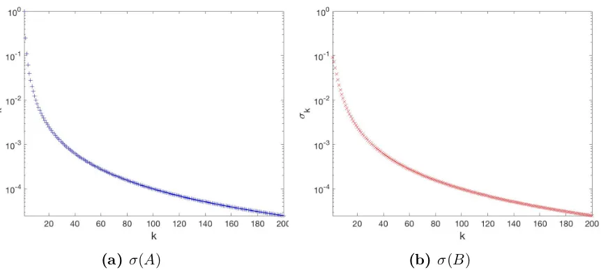
eigenfunctions since the decay rates of the singular values is the focus of this work. The first 200 singular values for A and B are plotted in Figure 4.1 on a semi-log scale. There we see how the early values decay quadratically. This decay continues on for the infinitely many singular values approaching zero.
4.2
Joint operator
(a) σ(A) (b) σ(B)
Figure 4.1: Singular values of individual operators
σ2φ=C∗Cφ =C∗(Aφ, Bφ) =A∗Aφ+B∗Bφ.
Using the analytical approach to calculating the singular values in Section 3.2.2, we apply the differential operators and their adjoints to arrive at an ODE,
σ2(LBL∗BLAL∗A)φ = (LBL∗B+LAL∗A)φ or,
σ2 φ(8)+ 2b2φ(6)+b4φ(4) = φ(4)+ 2b2φ(2)+b4φ+φ(4). (4.1)
As mentioned previously, some of our simplifications relied on the fact that LAL∗A and LBL∗B commute. We show that fact explicitly for this particular example.
LAL∗ALBLB∗h=LBL∗BL
∗
ALAh,
for all h∈ R(A∗A). Let us first expand the left hand side of the equation.
LAL∗ALBL∗Bh=LAL∗ALB h(2)+b2h
=LAL∗A h
(4)+ 2b2h(2)+b4h
=LA h(6)+ 2b2h(4)+b4h(2)
=h(8)+ 2b2h(6)+b4h(4).
Now, we expand the right hand side of the equation.
LBL∗BLAL∗Ah=LBL∗BLA h(2)
=LBL∗B h
(4)
=LB h(6)+b2h(4)
=h(8)+ 2b2h(6)+b4h(4).
Therefore, we can see that
LAL∗ALBLB∗h=LBL∗BL
∗
ALAh,
and so LAL∗A and LBL∗B commute.
φ(0) = φ(π) = 0, φ(2)(0) = φ(2)(π) = 0,
φ(4)(0) = φ(4)(π) = 0, φ(6)(0) = φ(6)(π) = 0.
The singular function, singular value pairs{(φk, σk)}∞k=1 satisfy equation (4.1) and the
corresponding boundary conditions. Even though this is a linear constant coefficient ODE, the eight roots of the characteristic polynomial make solving the boundary value problem analytically outside of the scope of this thesis. We therefore turn to the extension of the Galerkin method presented in section 3.2.3.
4.3
Joint singular values
The discretizations A(n) and B(n), described in Section 3.2.3, approximate the
operators A and B with orthonormal bases. Following the approach in [9, 11], we use orthonormal box functions as our bases. The interval domains Ωs = [0, π] and Ωt= [0, π] are divided intonsubintervals{Ω
(i)
s }and{Ω(ti)}with equal lengthshs and ht respectively. The orthonormal box functions are then
qi(s) =
h−s1/2, s ∈Ω(si) 0, else
pj(t) =
aij(n)=hs−1/2h−t1/2
Z
Ω(si)
Z
Ω(tj)
KA(s, t)dtds,
and similarly
bij(n) =hs−1/2h−t1/2
Z
Ω(si)
Z
Ω(tj)
KB(s, t)dtds.
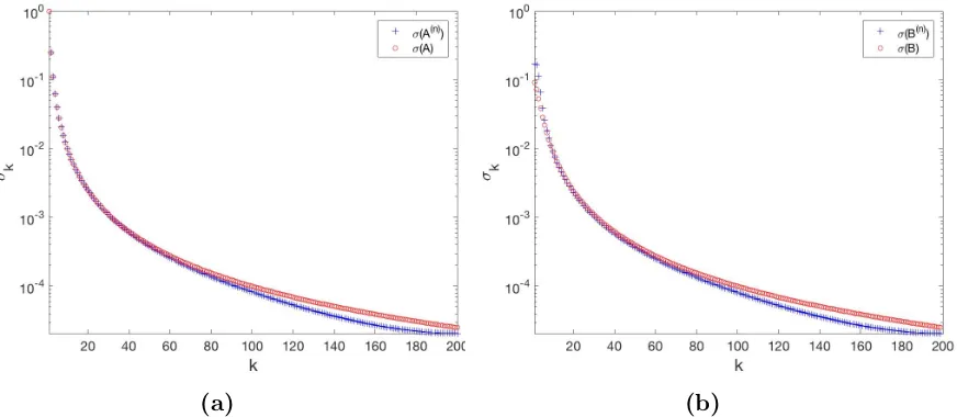
For b = π the analytically derived singular values are plotted with the numerical approximations on a semi-log scale in Figure 4.2. It should be noted that the use of orthonormal box functions in this Galerkin process is most effective for smooth kernels, as sharp features cannot be fully resolved with finitely many boxes.
(a) (b)
Figure 4.2: Analytical singular values and Galerkin method approximations using orthonormal box functions
The approximation C(n) to the joint operator C = A⊕B is formed by stacking
the matrices A(n) and B(n). i.e.
C(n) =
A(n)
B(n)
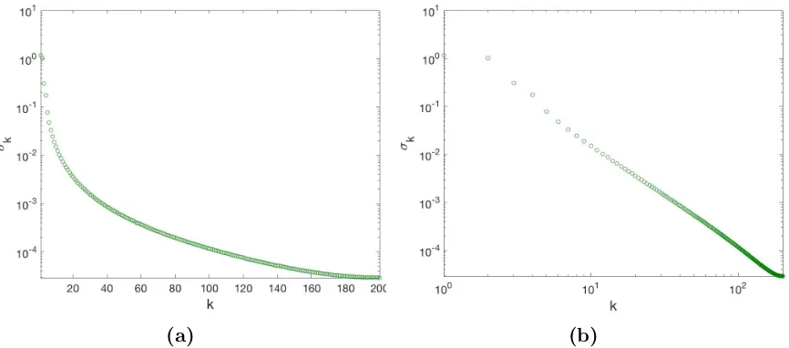
We approximate the continuous singular values ofC with the discrete singular values of C(n). The values σ(C(n)) are shown in Figure 4.3 on both a semi-log and log-log scale. Note that the first several singular values have a decay rate that is less than quadratic. Eventually the later ones decay quadratically to zero, but if we wished to consider a truncated SVD solution, we could include more singular values than if we used either model A or B individually.
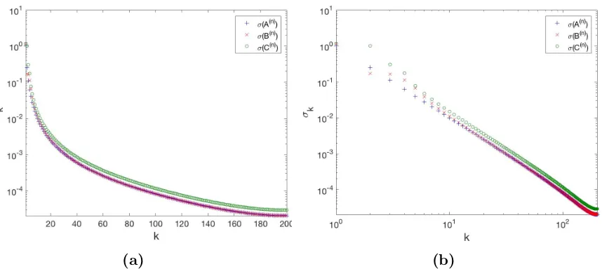
This modest improvement can clearly be seen in Figure 4.4, where we plot the singular values of the joint operator and singular values of the individual operators. We hypothesis that when we increase the complexity of the models under consider-ation there will be more substantial gains from joint inversion. We expect this to be especially true when considering models with complementary physics, such as ER and GPR.
(a) (b)
Figure 4.3: Approximate singular values of the joint operator C on a semi-log scale (a), and a log-log scale (b)
(a) (b)
Figure 4.4: Approximate singular values of the individual operators A and B, and the joint operator C on a semi-log scale (a), and a log-log scale (b)
CHAPTER 5
CONCLUSIONS AND FUTURE WORK
In this thesis, we explored inverse problems in both discrete and continuous settings with a focus on ill-conditioning and ill-posedness, respectively. We saw that the primary tool for analysis of discrete linear problems, the singular value decompo-sition, had an extension to continuous problems with compact linear operators, the singular value expansion. Using the SVE we were able to quantify the ill-posedness of continuous inverse problems by the decay rate of the singular values.
We then considered joint inverse problems. The first mention of joint inversion came in [22], where the authors used the singular value decomposition to determine the degree of ill-conditioning in discrete inverse problems. The authors demonstrated in several examples that combining two models in a joint inversion, and effectively stacking discrete linear models, improved the conditioning of the problem.
joint operator, we extended the Galerkin method given in [9, 18]. We the conditions necessary to capture the decay rate of the singular values by this approximation.
The results we have shown in this thesis are for simple cases. To increase the usefulness of the techniques presented here, we will need to construct more realistic and complicated models. The first step towards more realistic models will be the addition of another dimension. Green’s function solutions for partial differential equations will naturally require at least two variables related to the dimension of the problem and two associated dummy variables. Therefore, we will need to further extend our numerical techniques.
REFERENCES
[1] Richard C Aster, Brian Borchers, and Clifford H Thurber. Parameter estimation and inverse problems. Elsevier Academic Press, Amsterdam, The Netherlands,
2005.
[2] J.B. Conway. A Course in Functional Analysis. Graduate Texts in Mathematics. Springer New York, 1994.
[3] Dean G Duffy. Green’s Function with Applications. CRC Press, 2015.
[4] Andrew Geary. Setup of a dc resistivity survey, 2016.
[5] New Jersey Geological and Water Survey. Ground penetrating radar, 2005.
[6] Mark Gockenbach. Linear Inverse Problems and Tikhonov Regularization. The Mathematical Association of America, 2015.
[7] Mark S Gockenbach. Generalizing the gsvd. SIAM Journal on Numerical Analysis, 54(4):2517–2540, 2016.
[8] Paul Richard Halmos and Viakalathur Shankar Sunder. Bounded integral op-erators on L2 spaces. Ergebnisse Mathematik und GrenzGeb. Springer, Berlin,
1978.
[10] Per Christian Hansen. Rank-deficient and discrete ill-posed problems: numerical aspects of linear inversion, volume 4. Siam, 1998.
[11] Per Christian Hansen. Regularization tools version 4.0 for matlab 7.3. Numerical algorithms, 46(2):189–194, 2007.
[12] Per Christian Hansen. Discrete inverse problems: insight and algorithms. SIAM, 2010.
[13] Muneo Hori. Inverse analysis method using spectral decomposition of green’s function. Geophysical Journal International, 147(1):77–87, 2001.
[14] John D Jackson. Classical electrodynamics. John Wiley & Sons, Inc., New York, NY,, 1999.
[15] Michel Kern. Numerical Methods for Inverse Problems. John Wiley & Sons, 2016.
[16] Andreas Kirsch. An introduction to the mathematical theory of inverse problems, volume 120. Springer Science & Business Media, 2011.
[17] Rainer Kress, V Maz’ya, and V Kozlov. Linear integral equations, volume 82. Springer, 1989.
[18] Rosemary A Renaut, Michael Horst, Yang Wang, Douglas Cochran, and Jakob Hansen. Efficient estimation of regularization parameters via downsampling and the singular value expansion. BIT Numerical Mathematics, pages 1–31, 2016.
[20] Gilbert W Stewart. On the early history of the singular value decomposition. SIAM review, 35(4):551–566, 1993.
[21] Andre˘ı Nikolaevich Tikhonov, Vasili˘ı IAkovlevich Arsenin, and Fritz John. So-lutions of ill-posed problems, volume 14. Winston Washington, DC, 1977.
[22] K Vozoff and DLB Jupp. Joint inversion of geophysical data.Geophysical Journal International, 42(3):977–991, 1975.
![Figure 1.1: Electrical resistivity setup [4] (left) and ground penetrating radar[5] (right)](https://thumb-us.123doks.com/thumbv2/123dok_us/8919730.1840924/10.612.155.496.541.661/figure-electrical-resistivity-setup-ground-penetrating-radar-right.webp)
![Figure 3.2: Parametric curve defined by C(cos kx) for k ∈ [−5, 5]](https://thumb-us.123doks.com/thumbv2/123dok_us/8919730.1840924/38.612.151.487.104.377/figure-parametric-curve-dened-c-cos-kx-k.webp)