International Journal of Industrial Engineering Computations 6 (2015) 419–432
Contents lists available at GrowingScience
International Journal of Industrial Engineering Computations
homepage: www.GrowingScience.com/ijiec
Sensitivity analysis for casting process under stochastic modelling
Amit Kumara, Aman Kumar Varshneyb and Mangey Rama*
aDepartment of Mathematics, Graphic Era University Dehradun-248002, Uttarakhand, India
bDepartment of Mechanical Engineering, Graphic Era University Dehradun-248002, Uttarakhand, India
C H R O N I C L E A B S T R A C T
Article history:
Received September 14 2014 Received in Revised Format January 10 2015
Accepted January 30 2015 Available online February 2 2015
The present paper studies the reliability analysis of the casting process in foundry work using a probabilistic approach. As foundry industries in many developing countries suffer from poor quality of casting due to improper management, lack of resources and wrong working methods followed, which results in the decrement of productivity. Hence, to ensure the quality and productivity, favorable steps must be taken. The considered casting system has four main types of defects; namely mold shift, shrinkage, cold shut and blowholes. The complete casting system can fail due to the misalignment of the mold and combination of defects such as shrinkage and blow holes and can also fail by defects of shrinkage, blow holes and cold shut, simultaneously. The system is analyzed with the help of the supplementary variable technique and Laplace transformation. The availability, reliability, mean time to failure, sensitivity analysis and cost-effectiveness have been evaluated for the considered system. The results have been shown with the help of graphs, which predicts the behavior of the casting process system when any one of the defect or more than one defect appears.
© 2015 Growing Science Ltd. All rights reserved Keywords:
System Safety Sensitivity Analysis Casting Model Foundry Work Cost-effectiveness
1. Introduction
Casting is a process of pouring molten metal into a mold cavity and allowing it to solidify to obtain a desired product. By this process, intricate part can be given strength and rigidity, which is not frequently obtained by other methods.
Casting is generally based on a number of parameters such as mold, cavity, temperature of molten material and the most important is the experience of the designer. In casting many unquantifiable factors such as shrinkage, mold shift, cold shut, blow holes, porosity lead to conservative design rules. Unquantifiable factors are the ones with an unknown state of defect. The foundry industry suffers from poor quality and productivity due to a large number of parameters affecting it such as shortage of skilled labor, the poor working process followed, etc. Casting defect result in increased unit cost and lower morale of shop floor personnel. Close control and standardization of all aspects of production technique offer the best protection against casting defect. Due to a wide range of possible factors, reasonable classification of casting defect is difficult.
* Corresponding author.
The ability and efficiency of the casting process can be predicted by using the concept of reliability. Redundancies play essential role in increasing the reliability characteristics of systems (Ram & Kumar, 2014). High reliability of the system increases the efficiency of the production (Kumar & Ram, 2013). Reliability measures are the foremost concern in the planning, design, and operation of any system or equipment. Many researchers, including Pan (1997) discussed a multi-stage production system with one machine/tool in active state and n spares in standby state. Pan found that when the operating machine/tool breaks down, a switching device detects the machine failure via the sensor and the defective tool is replaced with a functional spare, so the system can resume its operations. Cavalca (2003) presented an availability optimization problem of an engineering system assembled in series configuration, by using genetic algorithm. Barabady and Kumar (2007) defined availability importance measures in order to calculate the criticality of each component or subsystem from the availability point of view and also demonstrated the application of such important measures for achieving optimal resource allocation to arrive at the best possible available. Filieri et al. (2010) focused on a CB software system that operates in safety-critical environment, where a relevant quality factor is the system reliability, defined as a probabilistic measure of the system's ability to successfully carry out its own task.
The other authors also (Ram & Singh, 2008, 2010; Ram, 2010, Ram et al., 2013) analyzed and evaluated the reliability measures for various engineering models under the concept of Gumbel-Hougaard family copula with different repair policies. Gupta and Sharma (1993) developed different models and analyzed the failure by computing the reliability measures such as availability, cost estimation, mean time to failure. Sutaria et al. (2012) discussed the capability to predict the temporal evolution of the interface and to identify that multiple hotspots is validated with an industrial aluminum-alloy lug casting. Venkatesan et al. (2005) discussed and developed a program for finite element modelling of casting solidification. The salient features of the program are: facility to incorporate latent heat through enthalpy method, incorporation of air gap by coincident node technique, ability to handle non-linear transient heat conduction through temperature dependent material properties, and object oriented programming. Tzong and Lee (1992) presented an investigation that an enthalpy formulation could be applied to the solidification process of an arbitrarily shaped casting in a mold-casting system. The effect of thermal contact resistance existing at the mold-casting interface was also studied. Joshi and Ravi (2010) defined shape complexity factor using weighted criteria based on part geometry parameters such as number of cored features, volume and surface area of the part, core volume, section thickness and draw distance.
element analysis to simulate the process of die-casting, and the quadratic response surface to represent the multidisciplinary optimization model of die-casting, in which they used evidence theory to represent the epistemic uncertainty. It is also well known that casting is an economical and efficient technology for producing metal parts. In the present scenario, casting technology is in its advanced form due the development of CAD engineers (Cleary, 2010). To prevent the defect and to increase productivity, various techniques like linear programing, Melt conditioner, Twin-roll strip casting and Auto-Cast-X software were used by different authors (Choudhari et al., 2014; Haghayeghi et al., 2010; Wang et al., 2010; Park & Yang, 2011).
Nowadays, several types of composite material exist, which play wide and extensive roles in manufacturing engineering components (Li et al., 2010; Thomas et al., 2014; Moses et al., 2014, Onat, 2010). Akhil et al. (2014) reported the cooling characteristics of cast components with varying section size and investigated how cooling rate and mechanical properties vary with varying section size. Tabibian et al. (2010) defined a thermo-mechanical fatigue criterion in order to predict the failure of cylinder heads issued with the lost foam casting process. Hamasaiid et al. (2010) proposed an analytical model to predict the time varying thermal conductance at the casting-die interface during solidification of light alloy during high pressure die-casting. System reliability occupies progressively more significant use in casting, manufacturing system, standby systems etc. Maintaining a high or required level of accuracy is often an essential requirement of the system. The study of the repairmen is an essential part of the repairable system and can affect the economy of the system directly or indirectly. Therefore, his/her action and work frames are vital in improving the reliability of repairable system.
2. Problem Statement
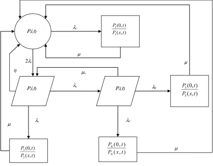
In the present paper, we deal with the reliability analysis of the casting process in foundry work. This research is intended to explain how much a defect can affect the casting system and its performance. Casting is done to provide strength and rigidity to the parts or system for bearing mechanical impacts. So, the reliability measures of the product are important criteria of judging the product life. There are four common defects, which affect the shape and size of the cast during casting, namely, mold shift, shrinkage, cold shut and blow holes. The state transition diagram of the proposed model has been shown in Fig. 1.
2.1Causes and Repairing Technique of Casting Defect
2.2.1 Mold Shift
It results in a mismatching of top and bottom part of a casting, usually at the parting line. It occurs due to the following reasons:
(a) Misalignment of pattern parts, due to worn or damaged patterns, (b) Misalignment of molding box or flask equipment.
This defect can be eliminated by ensuring proper alignment of the pattern, molding boxes and providing proper shrinkage and draft allowances etc.
2.2.2 Shrinkage
It is a defect when the thick metal solidifies. Generally, this defect occurs at hot spots. This is due to the following reasons:
(a) Improper location and size of gates and runners, (b) Incorrect metal composition,
This defect can be eliminated by the use of feeders and chills at proper locations to promote directional solidification.
2.2.3 Cold Shut
Cold shut is a crack with round edges form due to the low melting temperature or poor gating system. This is due to the following reasons:
(a) Too small gates,
(b) Too many restrictions on gating system, (c) Lack of fluidity in molten metal.
This defect can be eliminated by the proper use of a runner, riser and pouring temperature.
2.2.4 Blowholes
It is a defect which is caused by air and gases entrapped in the solidifying metal. This is due to the following reasons:
(a) Low gas permeability of the core sand, (b) Improper ramming.
This defect can be eliminated by changing the hardness of mold, use of appropriate sand with adequate green compact strength.
2.3 Inspection of Casting
Casting is inspected thoroughly to find the presence of internal flaws as well as well external defects. The various methods of inspecting casting are
(i) Visual examination, (ii) Sound or percussion test, (iii) Pressure test,
(iv) Magnetic and fluorescent powder inspection, (v) Radiographic examination,
(vi) Ultrasonic testing.
3. Assumptions and Notations
The following assumptions have been taken throughout the model: (i) Initially, the casting system is free from defects.
(ii) The casting system can consist of four defects. (iii) Each defect is either present or absent.
(iv) After repair or remedies, casting system is free from defects.
(v) When the major defect occurs in the casting system the cast component fails.
Further, the following notations are used:
Indicates that the system is in good condition,
Indicates that the system is in a degraded condition, Indicate that the system has failed condition,
P0(t) The probability that at time t system is working to full capacity,
P1(t) The probability that at time t system is failed due to defect of mold shift,
P2(t) The probability that at time t system is in a degraded state with blowholes defect,
P4(t) The probability that at time t system is in a degraded state with blowholes and cold shut defect,
P5(t) The probability that at time t system is failed due to defect of shrinkage, blowholes and cold shut,
P6(t) The probability that at time t system is failed due to defect of mold shift, blowholes and cold shut,
0
λ Failure rate of shrinkage and blowholes,
c
λ Failure rate of mold shift,
n
λ Failure rate of cold shut,
0
µ Repair rate of shrinkage, η Repair rate of blowholes,
µ Repair rate of remaining units, K1 Revenue per unit time,
K2 Service cost per unit time.
4. State Transition Diagram
Fig. 1. State Transition Diagram
5. Mathematical Formulation and Solution of the Model
By the probability considerations and continuity arguments we can obtain the following set of difference differential equations governing the present mathematical model
) t ( 0 P
) t ( 2
P P4(t)
0 λ 2
λc
µ
0 λ
c λ
n λ
µ
µ
η µ0
0 λ
( )
0 0 2
1,3,5,6 0
2
c( )
i( , )
i
P
t
P t
P x t dx
t
λ
λ
η
µ
∞ =
∂
+
+
=
+
∂
∑ ∫
(1)( )
2
0 0(
)
0 4(
)
2
0
P
t
P
t
P
t
t
η
λ
λ
n
=
λ
+
µ
+
+
+
∂
∂
(2)( )
2(
)
4 0
0
P
t
P
t
t
µ
λ
λ
c
=
λ
n
+
+
+
∂
∂
(3)( )
,
=
0
,
=
1
,
3
,
5
,
6
+
∂
∂
+
∂
∂
i
t
x
P
t
x
µ
i(4)
Boundary Conditions
( )
0
,
0(
)
1
t
P
t
P
=
λ
c (5)( )
0
,
0 2(
)
3
t
P
t
P
=
λ
(6)( )
0
,
0 4(
)
5
t
P
t
P
=
λ
(7)( )
0
,
4(
)
6
t
P
t
P
=
λ
c (8)Initial condition
( )
0
1
0
=
P
and all state probabilities are zero at t = 0. (9) Taking Laplace transformation from Eq. (1) to Eq. (8).(
0) ( )
0 21,3,5,6 0
2
c1
( )
i( , )
i
s
λ
λ
P
s
η
P s
µ
P x s dx
∞
=
+
+
= +
+
∑ ∫
(10)(
s +η
+λ
0 +λ
n) ( )
P2 s = 2λ
0P0(s) +µ
0P4(s) (11)(
s +µ
0 +λ
0 +λ
c) ( )
P4 s =λ
nP2(s) (12)( )
,
=
0
;
=
1
,
3
,
5
,
6
+
+
∂
∂
i
s
x
P
s
x
µ
i(13)
( )
0, 0( )1 s P s
P =
λ
c (14)(
0,)
0 2( )3 s P s
P =
λ
(15)(
0,)
0 4( )5 s P s
P =
λ
(16)(
0,)
4( )6 s P s
P =
λ
c (17)
Solving the Eqs. (10-13) with the help of Eqs. (14-17) and Eq. (9), one can obtain
( )
( )
( )
( )
s
T
H
s
T
s
T
H
H
s
s
P
cc 0 1 2 1 1 2 1
0
)
2
(
1
−
−
−
−
+
+
=
λ
λ
λ
(18)( )
01
( )
(
)
c
P s
P
s
s
λ
µ
=
−
(19)( )
0 0(
0 0)
2
4
2
P s
( )
s
cP
s
H
λ
+
µ
+
λ
+
λ
=
(20)( )
20 0(
0 0)
3
4
2
( )
(
)
c
P s
s
( )
0 0 44
2
nP s
( )
P
s
H
λ λ
=
(22)( )
20 05
4
2
( )
(
)
n
P s
P
s
s
H
λ λ
µ
=
−
(23)( )
0 06
4
2
( )
(
)
n c
P s
P
s
s
H
λ λ λ
µ
=
−
(24) where(
)
4 0 0 0 12
H
s
H
=
λ
η
+
µ
+
λ
+
λ
c,
(
)
4 0 0 0 2 22
H
s
H
=
λ
+
µ
+
λ
+
λ
c,
(
)
4 0 0 32
H
H
=
λ
λ
nλ
c+
λ
,
(
0 0)
00
4
=
(
s
+
η
+
λ
+
λ
n)
s
+
µ
+
λ
+
λ
c−
µλ
H
.The Laplace transformation of the probabilities that the system is in the up (i.e. good or degraded ) and down (i.e. failed) state at any time is as follows
( )
s
P
( )
s
P
( )
s
P
( )
s
P
up=
0+
2+
4 (25)( )
s P( )
s P( )
s P( )
s P( )
sPdown = 1 + 3 + 5 + 6 (26)
6. Particular Cases and Numerical Computations
6.1 Availability Analysis
Taking the values of different parameters as λc =0.2,λ0 =0.25,λn =0.1,µ =1,µ0 =η =1in Eq.
(25) taking inverse the Laplace transform, we get the availability of the system
( )
+
+
=
− −)
1391941091
.
0
sin(
205891151
.
0
)
1391194109
.
0
cos(
1793313070
.
0
8206686930
.
0
275 . 1 275 . 1t
e
t
e
t
P
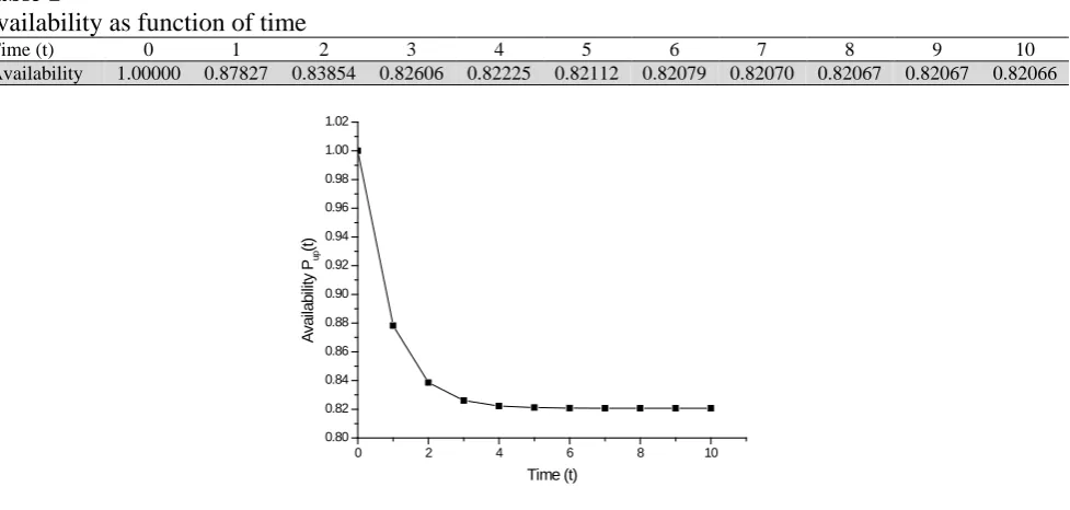
t t up (27)Now, taking t=0 to 10 units of time in Eq. (27), one can get the Table 1 and Fig. 2 respectively.
Table 1
Availability as function of time
Time (t) 0 1 2 3 4 5 6 7 8 9 10
Availability 1.00000 0.87827 0.83854 0.82606 0.82225 0.82112 0.82079 0.82070 0.82067 0.82067 0.82066
0 2 4 6 8 10
0.80 0.82 0.84 0.86 0.88 0.90 0.92 0.94 0.96 0.98 1.00 1.02 A va ila b ilit y P up (t ) Time (t)
6.2 Reliability Analysis
Taking all repair rates equal to be zero and failure rates λc =0.2,λ0 =0.25,λn =0.1in Eq. (25) and
then taking the inverse Laplace transform, the reliability of the system is given as
) 45 . 0 ( ) 35 . 0 ( )
525 . 0 ( )
7 . 0 (
2 428571429
. 1 ) 175 . 0 sinh( 857142857
. 2 571428571
. 1 )
(t e t e t t e t e t
R = − + − + − − − (28)
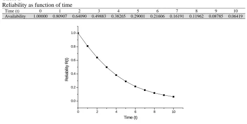
Now, taking t=0 to 10 units of time in the Eq. (28), we get the Table 2 and Fig. 3 respectively.
Table 2
Reliability as function of time
Time (t) 0 1 2 3 4 5 6 7 8 9 10
Availability 1.00000 0.80907 0.64090 0.49883 0.38265 0.29001 0.21606 0.16191 0.11962 0.08785 0.06419
0 2 4 6 8 10
0.0 0.2 0.4 0.6 0.8 1.0
R
e
lia
b
ilit
y R
(t
)
Time (t)
Fig. 3. Reliability as function of time
6.3 Mean Time to Failure (MTTF) Analysis
Taking all repair rates to be zero in Eq. (25) and taking s tends to zero; one can obtain the mean time to failure (MTTF) of the system as
)
)(
)(
2
(
2
)
)(
2
(
2
)
2
(
1
0 0
0 0
0 0
0
0
λ
λ
λ
λ
λ
λ
λ
λ
λ
λ
λ
λ
λ
λ
λ
+
+
+
+
+
+
+
+
=
c n c
n n
c c
MTTF
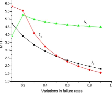
(29)Setting λc =0.2,λ0 =0.25,λn =0.1 and varyingλc, λ0, λnone by one from 0.1 to 0.9 in Eq. (29), we get
the following Table 3 and Fig. 4.
Table 3
MTTF as function of failure rates
Variation in 0.1 0.2 0.3 0.4 0.5 0.6 0.7 0.8 0.9
c
λ 4.72789 3.92290 3.36038 2.94261 2.61904 2.36058 2.14912 1.97278 1.823425
0
λ 5.83333 5.55555 4.10714 3.24444 2.67676 2.27629 1.97916 1.75018 4.53703
n
6.4 Sensitivity Analysis
The sensitivity of the reliability is a demanding input factor, which is most regularly defined as the partial derivative of the reliability with respect to that factor. This measure is then used to estimate the outcome of factor changes on the model result without requiring a full model solution for each factor change. These input factors are mostly failure rates. In similar fashion, one can define sensitivity of MTTF with respect to input factor.
0.2 0.4 0.6 0.8 1.0
1.0 1.5 2.0 2.5 3.0 3.5 4.0 4.5 5.0 5.5 6.0
λn
λc λ0
M
TTF
Variations in failure rates
0.2 0.4 0.6 0.8 1.0
-120 -100 -80 -60 -40 -20
0 w.r.t. λn
w.r.t. λ0
w.r.t. λc
S
ens
iti
vi
ty
of
M
T
T
F
Variation in failure rates
Fig. 4. MTTF as function of failure rates Fig. 5. Sensitivity of MTTF as function of failure rates
6.4.1 Sensitivity of MTTF
Sensitivity analysis for changes in MTTF resulting from changes in system parameters i.e. system failure ratesλc,λ0,λn. By Differentiating (29) with respect to failure ratesλc,λ0,λn respectively, we get the
values of
n c
MTTF MTTF
MTTF
λ λ
λ ∂
∂ ∂
∂ ∂
∂ ( )
, ) (
, ) (
0
.
Varying the failure rates one by one respectively as 0.1, 0.2, 0.3, 0.4, 0.5, 0.6, 0.7, 0.8, 0.9 in the partial derivatives of MTTF with respect to different failure rates, one can obtain the Table 4 and Fig. 5 respectively.
Table 4
Sensitivity of MTTF as function of failure rates Variation in
c
λ , λ0, λn c
MTTF
λ
∂ ∂( )
0 ) (
λ
∂ ∂ MTTF
n
MTTF
λ
∂ ∂( )
0.1 -113.94557 -15.27777 -2.59151
0.2 -35.21005 -11.57407 -1.56770
0.3 -16.90906 -7.62500 -1.04945
0.4 -9.90189 -5.24444 -0.75138
0.5 -6.49548 -3.78873 -0.56437
0.6 -4.58659 -2.85167 -0.43939
0.7 -3.41050 -2.21836 -0.35175
0.8 -2.63499 -1.77229 -0.28794
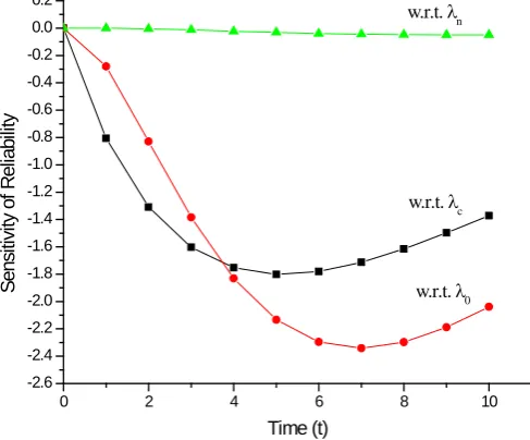
6.4.2 Sensitivity of Reliability
Here, authors perform a sensitivity analysis for changes in reliability resulting from changes in the system parametersλc,λ0andλnby taking all repair rates equal to zero and then taking the inverse Laplace transform in Eq. (25) and then differentiating it with respect to failure rates λc,λ0andλn respectively
and by putting λc=0.02, λ0=0.2, λn=0.15, get the values of
n c
t R t R t R
λ λ
λ ∂
∂ ∂ ∂ ∂
∂ ( )
, ) ( , ) (
0
.
Now, taking t=0 to 10 units of time in the partial derivatives of reliability with respect to different failure rates, one can obtain the Table 5 and Fig. 6 respectively.
Table 5
Sensitivity of Reliability as function of time
Time (t)
c
t R
λ
∂ ∂ ( )
0 ) (
λ
∂ ∂R t
n
t R
λ
∂ ∂ ( )
0 0 0 0
1 -0.80600 -0.28036 -0.00094
2 -1.30893 -0.82969 -0.00546
3 -1.60326 -1.38480 -0.01324
4 -1.75275 -1.83099 -0.02253
5 -1.80150 -2.13324 -0.031638
6 -1.78071 -2.29624 -0.039342
7 -1.71294 -2.34196 -0.045008
8 -1.61467 -2.29749 -0.048458
9 -1.49808 -2.18897 -0.049821
10 -1.37209 -2.03889 -0.049407
0 2 4 6 8 10
-2.6 -2.4 -2.2 -2.0 -1.8 -1.6 -1.4 -1.2 -1.0 -0.8 -0.6 -0.4 -0.2 0.0 0.2
w.r.t. λ0 w.r.t. λc w.r.t. λn
S
e
n
sit
iv
ity
o
f R
e
lia
b
ilit
y
Time (t)
Fig. 6. Sensitivity of Reliability as function of time
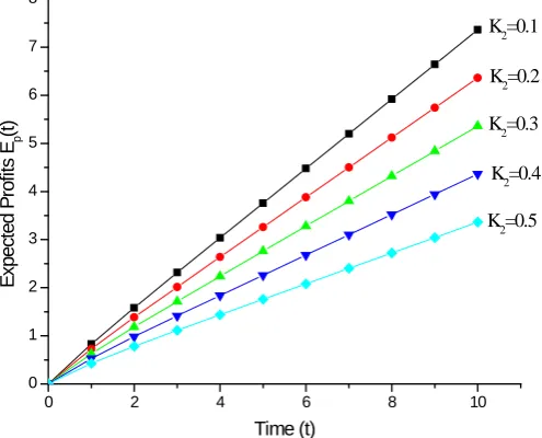
6.5 Expected Profit
The expected profit during the interval [0, t) is given as
1 2
0
( ) ( )
t
p up
Using Eq. (25), expected profit for the same set of parameters, we have
−
+
+
=
−−
2 275
. 1
275 . 1 1
)]
1391941091
.
0
sin(
205891151
.
0
)
1391194109
.
0
cos(
1793313070
.
0
820668693
.
0
[
)
(
tK
t
e
t
e
K
t
E
t
t p
(31)
Setting K1= 1 and K2= 0.1, 0.2, 0.3, 0.4, 0.5, respectively in Eq. (31), one can get the Table 6 and
correspondingly Fig.7.
Table 6
Expected profit as function of failure rates
Time (t) Expected Profits
1 . 0 2 =
K K2 =0.2 K2=0.3 K2 =0.4 K2 =0.5
0 0 0 0 0 0
1 0.82819 0.72819 0.62819 0.52819 0.42819 2 1.58290 1.38290 1.18290 0.98290 0.78290 3 2.31401 2.01401 1.71401 1.41401 1.11401 4 3.03781 2.63781 2.23781 1.83781 1.43781 5 3.75939 3.25939 2.75939 2.25939 1.75939 6 4.48032 3.88032 3.28032 2.68032 2.08032 7 5.20106 4.50106 3.80106 3.10106 2.40106 8 5.92175 5.12175 4.32175 3.52175 2.72175 9 6.64242 5.74242 4.84242 3.94242 3.04242 10 7.36309 6.36309 5.36309 4.36309 3.36309
0 2 4 6 8 10
0 1 2 3 4 5 6 7 8
K2=0.5 K2=0.4 K2=0.3 K2=0.2 K2=0.1
E
xpec
ted P
rof
its
E
p
(t
)
Time (t)
Fig.7. Expected profit as function of failure rates
7. Result Discussion
the system decreases precisely with the increment in time. By critically examining the Fig. 4, one can conclude that MTTF of the system decreases with respect to variation in failure rate of mold shift, Shrinkage and Blowholes and with respect to the failure rate of cold shut, first it increases then decreases. So the MTTF is the highest with respect to the failure rate of shrinkage and blowholes and the lowest with respect to the failure rate of Cold shut.
Fig. 5 shows the sensitivities of MTTF with respect to the failure rate of mold shift, shrinkage and blowholes and cold shut, which shows that it increases with the increment in failure rates. Critical observation of the graph point out that MTTF of the system is more sensitive again with respect toFailure rate of mold shift. Furthermore, the sensitivities of the system reliability with respect to the failure rate of mold shift, shrinkage and blowholes and cold shut are shown in Fig. 6. It reveals that sensitivity initially decreases with time passes. It is clear from the graph that system reliability is more sensitive with respect to failure rates of mold shift,shrinkage and blowholes. Keeping the revenue per unit time at one and varying service cost as 0.1, 0.2, 0.3, 0.4, and 0.5, one can obtain Fig. 7. It is very clear from the graph that the profit decreases as the service cost increases.
8. Conclusions
Most of the previous works were focused on finding process-related causes of individual defects, and optimized the parameter values to reduce the defects. In this work, the main focus was to predict that up to what extent our system could get affected if one of the above taken defects exists that is finally, explaining its dependency on parameter like mold shift, shrinkage, cold shut and blowholes. This will be helpful to the quality control department of casting industries to improve their productivity by minimizing the rejection of the cast parts. This work concludes the importance of the application of reliability in foundry work.Castings unfortunately can contain defects, which may render them unsuitable for service, resulting in higher costs and/or lower profits for the production foundry and delivery delays to the customer. It is also clear that the sensitivity of the system depends much more on system failure rates that is, the system can be made less sensitive by controlling its failures. It asserts that the result of this research will be useful in casting problems.
References
Akhil, K. T., Arul, S., & Sellamuthu, R. (2014). The Effect of Section Size on Cooling Rate,
Microstructure and Mechanical Properties of A356 Aluminium Alloy in Casting. Procedia Materials
Science, 5, 362-368.
Barabady, J., & Kumar, U. (2007). Availability allocation through importance measures. International Journal of Quality & Reliability Management, 24(6), 643-657.
Cavalca, K. L. (2003). Availability optimization with genetic algorithm. International Journal of Quality & Reliability Management, 20(7), 847-863.
Choudhari, C. M., Narkhede, B. E., & Mahajan, S. K. (2014). Casting Design and Simulation of Cover
Plate Using AutoCAST-X Software for Defect Minimization with Experimental Validation. Procedia
Materials Science, 6, 786-797.
Cleary, P. W. (2010). Extension of SPH to predict feeding, freezing and defect creation in low pressure
die casting. Applied Mathematical Modelling, 34(11), 3189-3201.
Filieri, A., Ghezzi, C., Grassi, V., & Mirandola, R. (2010). Reliability analysis of component-based systems with multiple failure modes. In Component-Based Software Engineering (pp. 1-20). Springer Berlin Heidelberg.
Gupta, P. P., & Sharma, M. K. (1993). Reliability and MTTF evaluation of a two duplex-unit standby system with two types of repair. Microelectronics Reliability, 33(3), 291-295.
Haghayeghi, R., Zoqui, E. J., Green, N. R., & Bahai, H. (2010). An investigation on DC casting of a
wrought aluminium alloy at below liquidus temperature by using melt conditioner. Journal of Alloys
Hamasaiid, A., Dour, G., Loulou, T., & Dargusch, M. S. (2010). A predictive model for the evolution of
the thermal conductance at the casting–die interfaces in high pressure die casting. International
Journal of Thermal Sciences, 49(2), 365-372.
Hojjati-Emami, K., Dhillon, B., & Jenab, K. (2012). Reliability prediction for the vehicles equipped with
advanced driver assistance systems (ADAS) and passive safety systems (PSS). International Journal
of Industrial Engineering Computations, 3(5), 731-742.
Joshi, D., & Ravi, B. (2010). Quantifying the Shape Complexity of Cast Parts. Computer-Aided Design and Applications, 7(5), 685-700.
Kumar, A., & Ram, M. (2013). Reliability measures improvement and sensitivity analysis of a coal
handling unit for thermal power plant. International Journal of Engineering-Transactions C: Aspects,
26(9), 1059.
Li, Q., Rottmair, C. A., & Singer, R. F. (2010). CNT reinforced light metal composites produced by melt
stirring and by high pressure die casting. Composites Science and Technology, 70(16), 2242-2247.
Mares, E., & Sokolowski, J. H. (2010). Artificial intelligence-based control system for the analysis of
metal casting properties. Journal of Achievements in Materials and Manufacturing Engineering,
40(2), 149-154
Moses, J. J., Dinaharan, I., & Sekhar, S. J. (2014). Characterization of Silicon Carbide Particulate
Reinforced AA6061 Aluminum Alloy Composites Produced via Stir Casting. Procedia Materials
Science, 5, 106-112.
Onat, A. (2010). Mechanical and dry sliding wear properties of silicon carbide particulate reinforced
aluminium–copper alloy matrix composites produced by direct squeeze casting method. Journal of
Alloys and Compounds, 489(1), 119-124.
Pan, J. N. (1997). Reliability prediction of imperfect switching systems subject to multiple stresses.
Microelectronics Reliability, 37(3), 439-445.
Park, Y. K., & Yang, J. M. (2011). Maximizing average efficiency of process time for pressure die casting
in real foundries. The International Journal of Advanced Manufacturing Technology, 53(9-12),
889-897.
Qi, H., & Li, Y. (2012). Metadynamic recrystallization of the as-cast 42CrMo steel after normalizing and
tempering during hot compression. Chinese Journal of Mechanical Engineering, 25(5), 853-859.
Ram, M. (2010). Reliability measures of a three-state complex system: a copula approach. Applications and Applied Mathematics: An International Journal, 5(10), 1483-1492.
Ram, M., & Kumar, A. (2014). Performance of a Structure Consisting a 2-out-of-3: F Substructure Under
Human Failure. Arabian Journal for Science and Engineering,39(11), 8383-8394.
Ram, M., & Singh, S. B. (2008). Availability and cost analysis of a parallel redundant complex system with two types of failure under preemptive-resume repair discipline using Gumbel-Hougaard family copula in repair. International Journal of Reliability, Quality and Safety Engineering, 15(04), 341-365.
Ram, M., & Singh, S. B. (2010). Analysis of a complex system with common cause failure and two types of repair facilities with different distributions in failure. International Journal of Reliability and Safety, 4(4), 381-392.
Ram, M., Singh, S. B., & Singh, V. V. (2013). Stochastic analysis of a standby system with waiting repair strategy. Systems, Man, and Cybernetics: Systems, IEEE Transactions on, 43(3), 698-707.
Sakallı, Ü. S., Baykoç, Ö. F., & Birgören, B. (2011). Stochastic optimization for blending problem in
brass casting industry. Annals of Operations Research, 186(1), 141-157
Soltani, R. (2014). Reliability optimization of binary state non-repairable systems: A state of the art
survey. International Journal of Industrial Engineering Computations, 5(3), 339-364.
Sutaria, M., Gada, V. H., Sharma, A., & Ravi, B. (2012). Computation of feed-paths for casting solidification using level-set-method. Journal of Materials Processing Technology, 212(6), 1236-1249.
Tabibian, S., Charkaluk, E., Constantinescu, A., Oudin, A., & Szmytka, F. (2010). Behavior, damage and fatigue life assessment of lost foam casting aluminum alloys under thermo-mechanical fatigue
Thomas, A. T., Parameshwaran, R., Muthukrishnan, A., & Kumaran, M. A. (2014). Development of
Feeding & Stirring Mechanisms for Stir Casting of Aluminium Matrix Composites. Procedia
Materials Science, 5, 1182-1191.
Tzong, R. Y., & Lee, S. L. (1992). Solidification of arbitrarily shaped casting in mold-casting system.
International Journal of Heat and Mass Transfer, 35(11), 2795-2803.
Venkatesan, A., Gopinath, V. M., & Rajadurai, A. (2005). Simulation of casting solidification and its grain structure prediction using FEM. Journal of Materials Processing Technology, 168(1), 10-15.
Wang, B., Zhang, J. Y., Li, X. M., & Qi, W. H. (2010). Simulation of solidification microstructure in
twin-roll casting strip. Computational Materials Science, 49(1), S135-S139
Wang, Y., Gong, C., Zhang, S., & Guo, H. (2010). Experimental study and numerical analysis on
heavy-duty cast steel universal hinged supports for large span structures. International Journal of Steel
Structures, 10(1), 99-114.
Wu, H., Li, D., Chen, X., Sun, B., & Xu, D. (2010). Rapid casting of turbine blades with abnormal film
cooling holes using integral ceramic casting molds. The International Journal of Advanced
Manufacturing Technology, 50(1-4), 13-19
Yang, Y., & Li, J. F. (2010). Study on mechanism of chip formation during high-speed milling of alloy
cast iron. The International Journal of Advanced Manufacturing Technology, 46(1-4), 43-50.
Yourui, T., Shuyong, D., & Xujing, Y. (2014). Reliability modeling and optimization of die-casting
existing epistemic uncertainty. International Journal on Interactive Design and Manufacturing
(IJIDeM), 1-7, DOI:10.1007/s12008-014-0239-y.
Zhang, L., & Li, L. (2013). Determination of heat transfer coefficients at metal/chill interface in the