21
International Journal of Advances in Engineering Research
STRUCTURED DATA PROCESSING QUALITY CONTROL
AND QUANTITY MODELLING OF PRODUCTS ON A
PRODUCTION LINE
Pushpendra Kumar Sharma1, Dr.B.Kumar2
1 Ph.D Research Scholar CMJ University Shillong, Meghalaya India 2Director RD Engineering College, Ghaziabad
ABSTRACT
The destination of this paper is structured data processing quality control and quantity modelling of products on a production line & to analyze how production system design, quality, and productivity of product are inter-related in small production systems. We develop a new process model for machines with both quality and operational failures, and we identify important deference’s between types of quality failures. We also develop models for two-machine systems, with in nite buers, buers of size zero, and -nite buers. We calculate total production rate, effective production rate (i e, the production rate of good parts), and yield. Numerical studies using these models show that when the first machine has quality failures and the inspection occurs only at the second machine, there are cases in which the effective production rate increases as buer sizes increase, and there are cases in which the effective production rate decreases for larger buers. We propose extensions to larger systems.The success of the Car Production System has prodding much research in manufacturing systems engineering. Productivity and quality have been extensively studied, but there is little research in their overlap.
Key words: Data Processing Quality, Productivity and Manufacturing System Design, buffer Design, Production, and Quantity of product.
INTRODUCTION
The recent popularity of Statistical Quality Control (SQC), Total Quality Management (TQM), and Six Sigma have demonstrated the importance of quality.
These two ends, productivity and quality, have been extensively studied and reported separately both in the manufacturing systems research literature and the practitioner literature, but there is little research in their intersection. The need for such work was recently described by authors from the GM Corporation based on their experience [13]. All manufacturers must satisfy these two requirements (high productivity and high quality) at the same time to maintain their competitiveness.
22
International Journal of Advances in Engineering Research
waste that would result from producing a series of defective items. Therefore jidoka a is a means to improve quality and increase productivity at the same time [23], [24]. But this statement is arguable: quality failures are often those in which the quality of each part is independent of the others. This is the case when the defect takes place due to common (or chance or random) causes of v aviations [16]. In this case, there is no reason to stop a machine that has made a bad part because there is no reason to believe that stopping it will reduce the number of bad parts in the future. In this case, therefore, stopping the operation does Sequence quality but it does reduce productivity. On the other hand, when quality failures are those in which once a bad part is produced, all
subsequent parts will be bad until the machine is repaired (due to special or assignable or systematic causes of Variations) [16], catching bad parts and stopping the machine as soon as possible is the best way to maintain high quality and productivity Non-stock or lean production is another popular buzzword in manufacturing systems engineering. Some lean manufacturing professionals advocate reducing inventory on the factory oor since the reduction of work-in-process (WIP) reveals the problems in the production lines [3].. In fact, Toyota recently changed their view on inventory and are trying to re-adjust their inventory levels [9]. What is missing in discussions of factory design, quality, and productivity is a quantitative model to show how they are inter-related. Most of the arguments about this are based on anecdotal evidence or qualitative reasoning that lacks a sound scientic quantitative foundation. The research described here tries to establish such a foundation to investigate how production system design and operation in Productivity and product quality by developing conceptual and computational models of two-machine-one-buer systems and performing numerical experiments.
HISTORY
23
International Journal of Advances in Engineering Research
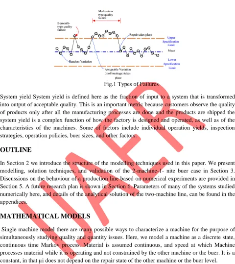
Fig.1 Types of Failures
System yield System yield is defined here as the fraction of input to a system that is transformed into output of acceptable quality. This is an important metric because customers observe the quality of products only after all the manufacturing processes are done and the products are shipped the system yield is a complex function of how the factory is designed and operated, as well as of the characteristics of the machines. Some of factors include individual operation yields, inspection strategies, operation policies, buer sizes, and other factors.
OUTLINE
In Section 2 we introduce the structure of the modelling techniques used in this paper. We present modelling, solution techniques, and validation of the 2-machine-1- nite buer case in Section 3. Discussions on the behaviour of a production line based on numerical experiments are provided in Section 5. A future research plan is shown in Section 6. Parameters of many of the systems studied numerically here, and details of the analytical solution of the two-machine line, can be found in the appendices.
MATHEMATICAL MODELS
Single machine model there are many possible ways to characterize a machine for the purpose of simultaneously studying quality and quantity issues. Here, we model a machine as a discrete state, continuous time Markov process. Material is assumed continuous, and speed at which Machine processes material while it is operating and not constrained by the other machine or the buer. It is a constant, in that µi does not depend on the repair state of the other machine or the buer level.
Figure 2 shows the proposed state transitions of a single machine with persistent-type quality failures. In the model, the machine has three states:
State 1: The machine is operating and producing good parts.
State -1: The machine is operating and producing bad parts, but the operator does not know this yet.
24
International Journal of Advances in Engineering Research
Fig.2 states of a machine
The machine therefore has two deferent failure modes (i.e. transition to failure states from state 1):
Operational failure: transition from state 1 to state 0. The
machine stops producing parts due to failures like motor burnout.
Quality failure: transition from state 1 to state -1. The
machine stops producing good parts (and starts producing bad parts) due to a failure like a sudden tool damage.
25
International Journal of Advances in Engineering Research
A flow (or transfer) line is a manufacturing system with a very special structure. It is a linear network of service stations or machines (M1, M2, ..., Mk ) separated by buer storages (B1, B2, ..., Bk 1 ). Material ows from outside the system to M1, then to B1, then to M2, and so forth until it reaches Mk , after which it leaves. Figure 3 depicts a flow line. The rectangles represent machines and the circles represent buffers.
Fig.3 five machine flow line
2-machine-1-buffer (2M1B) models should be studied first. Then a de-composition technique, that divides a long transfer line into multiple 2-machine-1-buer models, could be developed. (See [14].) Among the Various modelling techniques for the 2M1B case, including deterministic, exponential, and continuous models, the continuous material line model is used for this research because it can handle deterministic but different operation times at each operation. This is an extension of the continuous material serial line modelling of [10] by adding another machine failure state. Figure 4 shows the 2M1B continuous model where the machines, buer and discrete parts are represented as valves, a tank, and a continuous fluid.
26
International Journal of Advances in Engineering Research
INFINITE BUFFER CASE AN IN FINITE BUFFER CASE IS A SPECIAL
2M1B LINE IN WHICH THE SIZE OF THE BUFFER
(B) is in nite. This is an extreme case in which the first machine (M1) never suffers from block age. T o derive expressions for the total production rate and the effective production rate, we observe that when there is in finite buffer capacity between two machines (M1 , M2), the total production rate of the 2M1B system is a minimum of the total production rates of M1 and M2. The total production rate of machine i is given by (8), so the total production rate of the 2M1B system is the feature that M1 works on could take place at an inspection station at M2, and this inspection could trigger a repair of M1. (W e call this quality
information feedback. See Section 4.) In that case, the MTTD of M1 (and therefore f1) will be a function of the amount of material in the buffer. We return to this important case in Section 4
ZERO BUFFER CASE
The zero buffer case is one in which there is no buffer space between the machines. This is the other extreme case where block age and starvation take place most frequently .In the zero-bu er case in which machines have different operation times, whenever one of the machines stops, the other one is also stopped. In addition, when both of them are working, the production rate is min[µ1 ; µ2].Consider a long time interv al of length T during which M1 fails m1 times and M2 fails m2 times. If we assume that the average time to repair M1 is µ=r/ 1 and the average time to repair M2 is µ=r 2, then the total system downtime will be close to D =m/r1+m2 /r2. Consequently, the total up time will be Approximately
U = T - D = T (m1/r1+m2/r2)... (15)
27
International Journal of Advances in Engineering Research
The reduction of pi is explained in detail in [10]. The reductions of gi and fi are done for the same reasons. Table 2 lists the possible working states 1 and 2 of M1 and M2. The third column is the probability of finding the system in the indicated state. The fourth and fifth columns indicate the expected number of transitions to down states during the time interval from each of the states in column 1.
-Machine-1-Finite-Buffer Line The two-machine line is the simplest non-trivial case of a production line.In the existing literature on the performance evaluation of systems in which quality is not considered, two-machine lines are used in decomposition approximations of longer lines. (See [10].)We define the model here and show the solution technique in Appendix A
DEFINITION
28
International Journal of Advances in Engineering Research
MODEL DEVELOPMENT
Internal transition equations
When buffer B is neither empty nor full, its level can rise or fall depending on the states of adjacent machines. Since it can change only a small amount during a short time interval, it is natural to use differential equations to describe its behaviour. The probability of finding both machines at state 1 with a total storage level between x and x + x at time t + t is given by f (x; 1; 1) t, where
This is because if both machines are at state 1 at time t and the storage level is between x and x + (2 1), then there should be no failures before t + t to get f (x; 1; 1)t. The probability of not having any failures between t and t + t is
29
International Journal of Advances in Engineering Research
30
International Journal of Advances in Engineering Research
The probability that the first machine produces a non-defective part is then Y 1 = P 1 E=PT. Similarly, the probability that the second machine finishes its operation without adding a bad feature to a part is Y 2 = P2E=PT,
31
International Journal of Advances in Engineering Research
VALIDATION
The 2M1B systems with the same machine speed (1 = 2 ) are solved in Appendix A. As we have indicated, we represent discrete parts in this model as a continuous fluid and time as a continuous variable. We compare analytical and simulation results in this section. In the simulation, both material and time are discrete. Details are presented in [14].
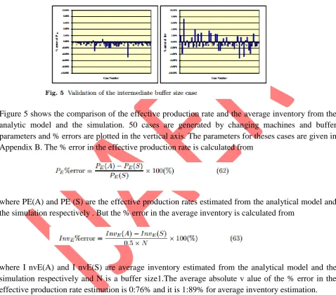
Figure 5 shows the comparison of the effective production rate and the average inventory from the analytic model and the simulation. 50 cases are generated by changing machines and buffer parameters and % errors are plotted in the vertical axis. The parameters for theses cases are given in Appendix B. The % error in the effective production rate is calculated from
where PE(A) and PE (S) are the effective production rates estimated from the analytical model and the simulation respectively . But the % error in the average inventory is calculated from
where I nvE(A) and I nvE(S) are average inventory estimated from the analytical model and the simulation respectively and N is a buffer size1.The average absolute v alue of the % error in the effective production rate estimation is 0:76% and it is 1:89% for average inventory estimation.
QUALITY INFORMATION FEEDBACKS
32
International Journal of Advances in Engineering Research
accumulate between an operation (M1) and the inspection of that operation (M2). All such material will be defective if a persistent quality failure takes place. In other words, if buffer is larger, there tends to be more material in the buffer and consequently more material is defective.
In addition it takes longer to have inspections after finishing operations. We can capture this phenomenon with the adjustment of a transition probability rate of M1 from state -1 to state 0. Let us define fq1 as a transition rate of M1 from state -1 to state 0 when
there is a quality information feedback and f 1 as the transition rate without the quality information feedback. The adjustment can be done in a way that the yield of M1 is the same as Zg1Zg1+Zb1
where Zb1: the expected number of bad parts generated by M1 while it stays in state -1. Zg1: the expected number of good parts produced by M1 from the mo-ment when M1 leaves the -1 state to the next time it arrives at state -1.1 Suppose that M1 has been in state 1 for a very long time. Then all parts in the buffer B are non-defective. Suppose that M1
33
International Journal of Advances in Engineering Research
Since the average inventory is a function of fq1and fq1is dependent on the average inventory, an iterative method is required to determine these values.
34
International Journal of Advances in Engineering Research
In this section, we perform a set of numerical experiments to provide intuitive insight into the behaviour of production lines with inspection. The parameters of all the cases are presented in Appendix B.
BENEFICIAL BUFFER CASE SYSTEM
Production rates having quality information feedback means having more inspection than otherwise. Therefore, machines tend to stop more frequently. As a result, the total production rate of the line decreases. However, the effective production rate can increase since added inspections prevent the making of defective parts. This phenomenon is shown in Figure 7. Note
that the total production rate PT without quality information feedback is consistently higher than PT with quality information feedback regardless of buffer size and the opposite is true for the effective production rate PE. Also it should be noted that in this case, both the total production rate and the effective production rate increase with buffer size, with or without quality information feedback.
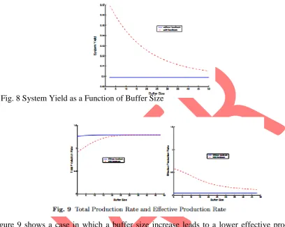
System yield and buffer size Even though a larger buffer increases both total and effective production rates in this case, it decreases yield. As explained in Section 4, the system yield is a function of the buffer size if there is quality information feedback. Figure 8 shows system yield decreasing as buffer size increases when there is quality information feedback. This happens because when the buffer gets larger, more material accumulates between an operation and the inspection of that operation. All such material will be defective when the first machine is at state -1 but the inspection at the first machine does not find it. This is a case in which a smaller buffer improves quality, which is widely believed to be generally true. If there is no quality information feedback, then the system yield is independent of the buffer size (and is substantially less).
HARMFUL BUFFER CASE
35
International Journal of Advances in Engineering Research
information feedback. The isolated production rate of the first machine is higher than that of the second machine:
Fig. 8 System Yield as a Function of Buffer Size
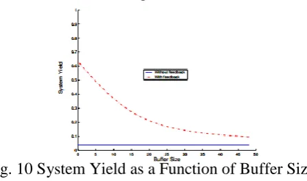
Figure 9 shows a case in which a buffer size increase leads to a lower effective production rate. Note that even in this case, total production rate monotonically increases as buffer size increases.
SYSTEM YIELD
The system yield for this case is shown in Figure 10.
Note that the yield decreases dramatically as the buffer size increases. In
this case, the decrease of the system yield is more than the increase of the total production rate so that the effective production rate monotonically decreases as buffer size gets bigger.
36
International Journal of Advances in Engineering Research
Fig. 10 System Yield as a Function of Buffer Size
increase the Mean Time to Quality F ailure (MTQF) (i.e. decrease g). On the other hand, the inspection policy aims to detect bad parts as soon as possible and prevent their flow toward downstream operations. More rigorous inspection decreases the mean time to detect (MTTD) (i.e. increases h and therefore increases f ). It is natural to believe that using only one kind of method to achieve a target quality level would not give the most cost efficient quality assurance policy . Figure 11 indicates that the impact of individual operation stabilization on the system yield decreases as the operation becomes more stable. It also shows that effect of improving inspection (MTTD) on the system yield decreases. Therefore, it is optimal to use a combination of both methods to improve quality.
HOW TO INCREASE PRODUCTIVITY & PRODUCTION OF A PRODUCT
Improving the stand-alone throughput of each operation and increasing the buffer space are typical ways to increase the production rate of manufacturing systems. If operations are apt to have quality failures, however, there may be other ways to increase the effective production rate: increasing the yield of each operation and conducting more extensive inspections. Stabi-lizing operations, thus improving the yield of individual operations, will increase effective throughput of a manufacturing system regardless of the type of quality failure. On the other hand, reducing the mean time to detect (MTTD) will incr ease the effective production rate only if the quality failure is persistent but it will decrease the effective production rate if the quality failure is Bernoulli. This is because the quality of each part is independent of the others when the quality failure is Bernoulli. Therefore, stopping the line does not reduce the number of bad parts in the future. In a situation in which machines produce defective parts frequently and inspection is poor, increasing inspection reliability is more
effective than increasing buffer size to boost the e
37
International Journal of Advances in Engineering Research
Fig. 12 Mean Time to Detect and Effective Production Rate
FUTURE SCOPES
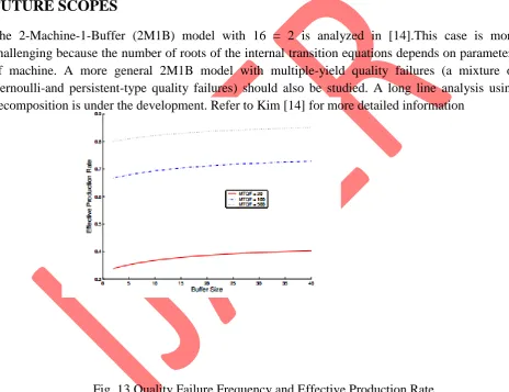
The 2-Machine-1-Buffer (2M1B) model with 16 = 2 is analyzed in [14].This case is more challenging because the number of roots of the internal transition equations depends on parameters of machine. A more general 2M1B model with multiple-yield quality failures (a mixture of Bernoulli-and persistent-type quality failures) should also be studied. A long line analysis using decomposition is under the development. Refer to Kim [14] for more detailed information
Fig. 13 Quality Failure Frequency and Effective Production Rate
REFERENCES
1) Alles M, Amershi A, Datar S, and Sarkar R (2000) Information and incentive effects of inventory in JIT production. Management science 46 (12): 1528{1544.
2) Bester field D H, Bester field-Michna C, Bester eld G, and Bester eld-Sacre M, (2003) Total quality management. Prentice Hall.
3) Black J T (1991) The design of the factory with a future. McGraw-Hill.
38
International Journal of Advances in Engineering Research
research to improve the design of a printer production line. Interfaces 28 (1): 24{26.
6) Buzacott J A and Shantikumar J G (1993) Stochastic models of manufacturing systems. Prentice Hall.
7) Cheng C H, Miltenburg J, and Motwani J (2000) The effect of straight and U shaped lines on quality . IEEE Transactions on Engineering Management 47 (3):321-334.
8) Dallery Y. and Gershwin S B (1992) Manufacturing flow line systems: a review of models and analytical results. Queuing Systems Theory and Applications 12:3{94.
9) Fujimoto T (1999) The evolution of a manufacturing systems at Toyota. Oxford University Press.
10)Gershwin S B (1994) Manufacturing systems engineering. Prentice Hall.
11)Gershwin S B (2000) Design and Operation of Manufacturing Systems | The Control-Point Policy . IIE Transactions 32 (2): 891-906.
12)Gershwin S B and Schor J E (2000) E cient algorithms for buffer space allocation. Annals of Operations Research 93: 117-144.
13)Inman R R, Blumenfeld D E, Huang N, and Li J (2003) Designing production systems for quality: research opportunities from an automotive industry perspective. International journal of production research 41 (9): 1953{1971.
14)Kim J (2004) Integrated Quality and Quantity Modeling of a Production Line.Massachusetts Institute of Technology Ph.D. thesis in preparation.
15)Law A M, Kelton D W, Kelton W D, and Kelton D M(1999) Simulation modeling and analysis. McGraw-Hill.
16)Ledolter J and Burrill C W (1999) Statistical quality control. John Wiley & Sons.
17)Monden Y (1998) Toyota production system | An integrated approach to Just-In-Time. EMP Books, 1998.
18)Montgomery D C (2001) Introduction to statistical quality control 4th edition.John Wiley & Sons.
19)Pande P and Holpp L (2002) What is six sigma? McGraw-Hill.
20)Phadke M (1989) Quality engineering using robust design. Prentice Hall.
21)Raz T (1986) A survey of models for allocating inspection effort in multistage production systems. Journal of quality technology 18 (4): 239{246.
22)Shin W S, Mart S M, and Lee H F (1995) Strategic allocation of inspection stations for a flow assembly line: a hybrid procedure. IIE Transactions 27: 707{715.
23)Shingo S, (1989) A study of the Toyota production system from an industrial engineering viewpoint. Productivity Press.
24)Toyota Motor Corporation (1996) The Toyota production system.
25)Wein L, (1988) Scheduling semiconductor wafer fabrication. IEEE Transac-tions on semiconductor manufacturing 1(3): 115{130.