* Corresponding author.Tel.: (+98)9141009365; E-mail address:[email protected](A. Rastbood).
Journal Homepage: ijmge.ut.ac.ir
IJMGE 51-1 (2017) 71–78 DOI: 10.22059/ijmge.2017.223801.594650
Prediction of structural forces of segmental tunnel lining using FEM based
artificial neural network
Armin Rastbood
a*, , Abbas Majdi
a, Yaghoob Gholipour
b a School of Mining, College of Engineering, University of Tehran, Tehran, Iran. bSchool of Civil, College of Engineering, University of Tehran, Tehran, Iran.ABSTRACT
The critical parameters in investigating the performance of designed support system of tunnels are the structural forces i.e. peak values of axial and shear forces, and moments. In this research, a complete database was firstly prepared using finite element method. Using finite element models, we modeled the segmental tunnel lining that was composed of 5+1 concrete segments in one ring. Then, an artificial neural network (ANN) model of multi-layer perceptron was developed to estimate the lining structural forces. To do this, the number of neurons and their arrangement were optimized based on the obtained minimum values from the root mean square error (RMSE). To prove the efficiency of the developed ANN model, we calculated the coefficient of efficiency (CE), determination coefficient (R2), variance account for (VAF), and RMSE values. The results demonstrated a promising precision and high efficiency of the presented ANN method for estimating the structural forces of tunnel lining composed of concrete segments instead of alternative costly and tedious solutions. Finally, the sensitivity analysis showed that among the input variables, the tunnel cover is the most influencing variable on the lining structural forces. However, other input variables, i.e. lateral earth pressure and key segment position were the second important variables affecting the induced stresses on tunnel lining.
Keywords : Artificial neural network, Lining, Multi-layer perceptron, Segment, Tunnel
1.
Introduction
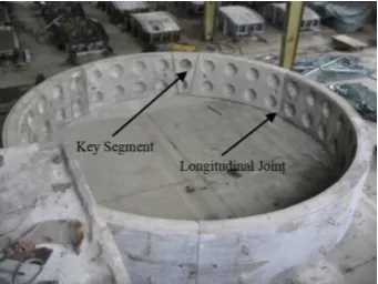
Support system of tunnels that are excavated by shield TBMs (Tunnel Boring Machine) is generally composed of segments with reinforced concrete (RC). Assembling these concrete segments inside the tunnel excavation shield forms the tunnel support rings. Construction of RC segments is a crucial step in tunnel construction procedure [1-4]. Due to the simplicity in installation and the assembling operation of a ring, one segment has to be designed smaller than the others which is called the key segment that is installed at the end of the ring. Fig 1 shows the assembled ring of RC segments in segment manufacturing factory [5]. Design methods of RC segments can be classified in three approaches: laboratory or experimental methods, closed form solutions or analytical methods, and numerical methods.
Analytical solutions have been extended from the beginning of underground openings designing until now [1, 6-16]. Some analytical solutions are restricted either to only elastic behavior of materials or only to shallow tunnels. Some others, taking into consideration few simple assumptions with reduced stiffness of segmental support ring with respect to the continuous ring without longitudinal joints and do not consider key segment shape and size in comparison with other segments in the assembled ring.
Recently, some design and monitoring processes of RC segmental tunnel lining behaviour were done through laboratorial experiments [6; 21; 22; 26; 29; 30; 32]. The experimental approaches are very reliable methods than analytical and numerical methods, but these methods are often expensive and tedious.
To overcome the experimental and analytical defects, numerical solutions have been extended widely in last decades [1; 2; 3; 7; 9; 13].
However, the numerical solutions are often time-consuming and need more detailed data that could be unidentified during analysis. The output results of numerical attempts should be verified by either experimental or analytical solutions or by in-field monitoring results. In last years, innovative methods like Artificial Neural Network (ANN) have been applied as a prediction tool to study the complex problems. Such approaches have been extended widely in geotechnical and geomechanical engineering problems [4; 5; 12; 14; 16; 17; 18; 19; 20; 23; 27; 28; 31]. As the above mentioned defects of the triple individual approaches reveal, ANN methods seem to be new alternative solutions. Estimation of structural forces in RC segments of tunnel lining structure using ANN has not been studied in detail as of yet. In this paper, ANN method was applied to estimate the structural forces of RC segments in tunnel lining structure based on the results of finite element method. Sensitivity analysis of variables was performed to assess their influence on the output results. Finally the applicability and efficiency of the designed ANN model were evaluated using RMSE (%), R2, VAF (%), and CE indices.
2.
The Concept of artificial neural network
Artificial neural networks are consisted of many data processing units called neurons. By using neurons, the network are capable to simulate the operation of human brain nature on the basis of trial and error method [34, 43]. In a common ANN model, there is a huge number of interconnections among the neurons. Generally, an ANN model is mostly composed of three layers named: input layer, hidden layer(s) and output layer. Schematic view of a usual ANN is illustrated in Fig. 2.
Article History:
Fig. 1. Assembled ring from RC segments in segment manufacturing factory, Tehran metro project, Line 4
Hidden layer(s) is the important layer of one neural network model because the main calculation phase is performed in it. Neurons in each layer are linked to the neurons of nearby layer with a coefficient named weight (w). Outputs of input layer is as input signal for the hidden layer(s) and the similar rule is governed between hidden layer(s) and output layer, respectively. Optimized number of neurons and hidden layers are calculated based on the trial and error rule and the goal error value [34].
Fig. 2. An illustration of a usual ANN [10]
ANN is trained at first and consequently tested and verified by other different data. In training process, inputs are entered and outputs values are determined. Then the error between the real and predicted values is calculated. Base on calculated error value, the weights are adjusted by starting from the last output layer towards the first input layer; this procedure is known as back propagation algorithm. Back propagation algorithms are potent implements for models with prediction aims [10]. Perceptron Neural network model was proposed by Rosenblatt [24]. Multi-layer perceptron NN, on the other hand, was improved and proposed by Rumelhart [25]. In this model, the input layer normalizes the input values. This type of data preparation and normalization improves the network performances, because of more homogeneous scattering of normalized data, as illustrated in Fig 3. This method of data normalization has been utilized by many researches [11; 15; 28]. Multi-layer perceptron (MLP) is an adjustment of the linear standard perceptron which can separate data without capability of linearly separation [8].
Fig. 3. Homogeneous distribution of data after normalization process [11].
3.
Database
3.1.Numerical analysis
Application of NN model of multi-layer perceptron for estimation of structural forces of RC segments in tunnel lining, requires to supply a comprehensive database. To do this, we used the resulted values from finite element (FE) analysis (ABAQUS 2014, Version 6.14. Abaqus, Inc., Pawtucket, Providence, R.I.). In the designed numerical model of tunnel lining, the support structure in one ring consisted of 5+1 segments. The engineering and geometrical characteristics of RC segments are summarized in Table 1. From size point of view, in one ring, five RC segments (A2-A6) were almost similar to each other. To decrease the total calculation time of numerical modelling, soil elements are neglected in the FE model. Therefore, the beam-spring method was applied to model the structure of tunnel lining [1, 2]. In this method the effects of soil body on the exterior side of tunnel lining and interaction between them were simulated using tangential and radial springs. Because of their negligible effects with respect to radial springs, tangential springs were neglected. Stiffness of soil radial springs is calculated using the following Eq. (1) [49]:
1 .
. R
E A K
(1) Where, K is stiffness of radial spring, E is Young modulus of soil, ν is poison’s ratio of soil, R is tunnel radius, and A is effective area on the exterior side of lining structure that is subjected to applied load because of the soil, and calculated by Eq. (2):
b
R
A
.
(2)Where, θ is the angle in terms of radial between 2 successive radial springs, and b is effective area of each spring in tunnel longitudinal direction. Figs. 4(a)-(b) show the perspective and non-perspective views of an assembled ring under soil radial springs. In structural modelling, load from surrounding ground was applied radially towards tunnel lining, Fig. 5. Normal radial stresses applied on tunnel lining structure are calculated by Eq. (3):
(3)
2 2
0 0cos 0sin
n v h
Where, σn0 is the normal stress, σv0 is the vertical stress, σh0 is the horizontal stress, and θ is radial angle measured from tunnel bottom [1].
A. Rastbood et al. / Int. J. Min. & Geo-Eng. (IJMGE), 51-1 (2017) 71-78 73
(b) Perspective view
Fig. 4. Assembled ring under soil radial springs in x (radial) direction
Fig. 5. Applied radial load from the surrounding ground on tunnel lining exterior side
Table1. Engineering and geometrical characteristics of concrete segments
Seg
men
t N
o.
Engineering properties Geometrical properties
E(GP
a)
ν
(p
oiss
on
ra
tio
)
ρ
(kg
/m
3)
M
at
er
ial
be
ha
vio
ur
t (Thic
kn
ess
-c
m
)
C
ent
ra
l ang
le
(
°)
A1(key
segment) 25 0.15 2350
CDP (Concrete
damage plasticity)
30 30
A2-A6 66
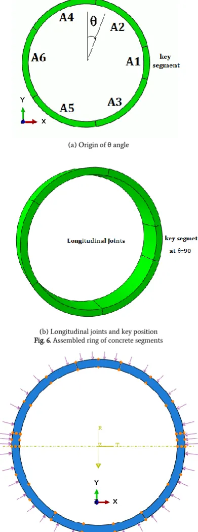
3D solid elements were used to model the segments of a ring. After assembling the concrete segments, the plane strain conditions were applied to the model. In current numerical models, it was assumed that the origin of angle in model plane is positioned at the tunnel crown (see Fig. 6(a)). Joints between two adjacent segments named longitudinal joints. Fig. 6(b) shows longitudinal joints of assembled segments in one individual ring and the position of key segment at θ=90°. The assembled ring is representative of support structure of tunnel lining. Hard contact was supposed for six concrete to concrete contact surfaces with frictional penalty coefficient of 0.4.
3.2.Data preparation
The model at first was solved for tunnel overburden H= 5m, K=0.47 (lateral earth pressure) and θ=0°. Then both H and K parameters were
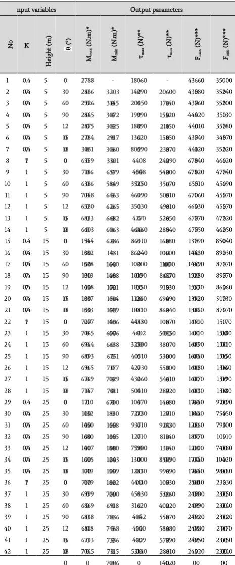
kept constant and θ value changed to 30°, 60°, 90°, 120°, 150° and 180°, respectively. This sort of variation for input parameters, was considered for H=15 m, 25m and K=0.47 and 1.0 (Hydrostatic condition of the ground). Straight type of longitudinal joints, i.e. parallel with z-axis were considered. Key segment positions at 210°, 240°, 270°, 300° and 330° were neglected because of the axisymmetric geometry of assembled ring. Tunnel lining under the ground load is shown in Fig. 7. Finally, 42 data sets were obtained. Input data variables and resulted output are presented in Table 2. Fig 8 shows the output values resulted for shear and axial force and moment quantities for an arbitrary section of the modelled ring.
(a) Origin of θ angle
(b) Longitudinal joints and key position Fig. 6. Assembled ring of concrete segments
Fig. 8. Resulted axial force (N) and shear force (N) and moment (N.M) for an arbitrary section of a segment in an assembled ring
3.3.Data normalization
To increase the processing and convergence rate of ANN during training process and to minimize the prediction error, raw data obtained from numerical models must be normalized [49].
Before commencing the modelling, all data must be filtered and the outliers should be deleted. Normalization of data proportionate all the variables with respect to each other. Traditionally, to normalize the data, the aforementioned approach means to fit the data within unity (1), herein all data values will be in the range of zero to unity. Unity-based normalization relation follows the Eq. 4 [50]:
min max min
u
u
u
u
u
Norm
(4)Where, u is any raw data, uNorm is the normalized data, umin is the minimum value of data and umax is the maximum value of data.
4.
Design of optimum and model
The data obtained from FE models were applied to make the multi-layer perceptron model for prediction aim. In this study, all data were divided in 3 parts: training data (70% of total data), testing data (20% of total data) and validation data (10% of total data).
Optimized structure of NN model, i.e. arrangement of neurons in hidden layers and the number of hidden layers, should be calculated on the basis of trial and error rule.
At first, optimized number of neurons was calculated based on the obtained values of root mean square error (RMSE). To do this, different variety of neurons were embedded in hidden layers of the model and RMSE value was calculated according to Eq. 5:
N i k ku
u
N
RMSE
1 2ˆ
.
1
(5)Where, u ̂k and
u
k are the kth predicted and observed values of target,respectively, and N is the number of observations for which the error has been computed.
The results are illustrated in Fig. 9. It can be concluded that the minimum value of RMSE was obtained by 6 number of neurons. Thereafter, these neurons must be arranged in one or two hidden layers. Flood et al. [47] stated that MLP model with two minimum hidden layers provides more flexibility for modelling complex problems.
Table 2. Raw data resulted from the finite element method
nput variables Output parameters
N
o K
H ei gh t ( m ) θ ( °) Mm ax (N .m )* Mm in (N .m )*
τmax
(N
)*
*
τmin
(N
)*
*
Fmax
(N
)***
Fmin
(N
)***
1 0.4 7
5 0 2788 0 -3203 0 18060 0 -20600 0 43660 0 35000 0 2 0.4
7
5 30 2836 0 -3145 0 14290 0 -17140 0 43580 0 35240 0 3 0.4
7
5 60 2926 0 -3072 0 20650 0 -15520 0 43760 0 35200 0 4 0.4
7
5 90 2845 0 -3025 0 19990 0 -21150 0 44420 0 35130 0 5 0.4
7
5 12 0 2875 0 -2917 0 18890 0 -15850 0 44010 0 35780 0 6 0.4
7
5 15 0 2784 0 -3060 0 13620 0 -23370 0 43740 0 34870 0 7 0.4
7
5 18 0 3031 0 -3301 0
80590 -24290 0 44120 0 35220 0 8 1 5 0 6559
0 -6579 0 4408 00 -54200 0 67840 0 46620 0 9 1 5 30 7186
0 -5849 0 4548 00 -35670 0 67820 0 47740 0 10 1 5 60 6386
0 -6463 0 35250 0 -50510 0 65510 0 45690 0 11 1 5 90 7048
0 -6265 0 46990 0 -49810 0 67060 0 45570 0 12 1 5 12
0 6520 0 -6682 0 35030 0 -52650 0 66930 0 45570 0 13 1 5 15
0 6833 0 -6063 0 4270 00 -28540 0 67770 0 47220 0 14 1 5 18
0 6603 0 -6286 0 46460 0 -16880 0 67750 0 46250 0 15 0.4
7
15 0 1544 00 -1431 00 86310 0 -10600 00 13790 00 85040 0 16 0.4
7
15 30 1382 00 -1640 00 86240 0 -11000 00 14430 00 89230 0 17 0.4
7
15 60 1528 00 -1488 00 10200 00 -86570 0 14490 00 87770 0 18 0.4
7
15 90 1313 00 -1721 00 10190 00 -91530 0 15280 00 89770 0 19 0.4
7
15 12 0 1498 00 -1514 00 10350 00 -69490 0 15530 00 86960 0 20 0.4
7
15 15 0 1337 00 -1679 00 11260 00 -86240 0 13920 00 91730 0 21 0.4
7
15 18 0 1533 00 -1436 00 10810 00 -10870 00 13860 00 87670 0 22 1 15 0 7277
0 -6976 0 44330 0 -50450 0 16910 00 15170 00 23 1 15 30 7065
0 -6638 0 4602 00 -38070 0 16810 00 15180 00 24 1 15 60 6944
0 -6751 0 32500 0 -53000 0 16890 00 15210 00 25 1 15 90 6893
0 -7177 0 40510 0 -55300 0 16840 00 15150 00 26 1 15 12
0 6965 0 -7029 0 42730 0 -54610 0 16880 00 15160 00 27 1 15 15
0 6769 0 -7011 0 43260 0 -28720 0 16870 00 15190 00 28 1 15 18
0 7147 0 -6700 0 50410 0 -14680 0 16830 00 15180 00 29 0.4
7
25 0 1710 00 -1830 00 10470 00 -12710 00 17640 00 97890 0 30 0.4
7
25 30 1132 00 -1558 00 72730 0 -92430 0 11440 00 75450 0 31 0.4
7
25 60 1450 00 -1355 00 93710 0 -81140 0 12860 00 79300 0 32 0.4
7
25 90 1680 00 -1880 00 12710 00 -13140 00 18970 00 10910 00 33 0.4
7
25 12 0 1407 00 -1243 00 75900 0 -85090 0 12100 00 74880 0 34 0.4
7
25 15 0 1605 00 -1999 00 13000 00 -99690 0 17340 00 10420 00 35 0.4
7
25 18 0 1719 00 -1822 00 12830 00 -10730 00 17640 00 98680 0 36 1 25 0 7179
0 -7290 0 44410 0 -53360 0 25010 00 23230 00 37 1 25 30 6999
0 -6918 0 45830 0 -40220 0 24900 00 23250 00 38 1 25 60 6869
0 -7036 0 31620 0 -55870 0 24990 00 23240 00 39 1 25 90 6838
0 -7468 0 4042 00 -58480 0 24920 00 23220 00 40 1 25 12
0 6818 0 -7336 0 4540 00 -57790 0 24980 00 23170 00 41 1 25 15
0 6733 0 -7315 0 4299 00 -28810 0 24950 0 23250 00 42 1 25 18
0 7045 0 -7006 0 53140 0 -14020 0 24920 00 23240 00
A. Rastbood et al. / Int. J. Min. & Geo-Eng. (IJMGE), 51-1 (2017) 71-78 75
Fig. 9. Optimum number of neurons in hidden layer(s) based on minimum value for RMSE
It can be concluded that model has the best efficiency in 3-4-2-1 for neurons arrangement based on the minimum RMSE value. Finally, schematic architecture of optimized network is shown in Fig. 10.
Table 3. Optimum arrangement of neurons in hidden layers
RMSE (Transfer Function:
LOGSIG) RMSE
(Transfer Function: TANSIG) Network
arrangement No.
0.10 0.04
3-6-1 1
0.11 0.51
3-1-5-1 2
0.08 0.07
3-2-4-1 3
0.04 0.02
3-3-3-1 4
0.01 0.01
3-4-2-1 5
0.03 0.05
3-5-1-1 6
Fig. 10. Architecture of Optimized MLP neural network
5.
Results and discussion
5.1.Model performance evaluation
Performance of artificial neural network should be assessed in predicting the capability of outputs. Therefore, four performance indices including determination coefficient (R2), variance account for (VAF), coefficient of efficiency (CE) and root mean square error (RMSE) were selected and calculated using testing data sets. These data sets were selected randomly from the database and were not included in training phase. VAF and CE values were calculated from Eqs. (6)–(7):
k k k
u u u VAF
var ˆ var 1
100 (6)
N k
k k N k
k k
u u
u u
CE
1 2 1
2
ˆ ˆ ˆ
1 (7)
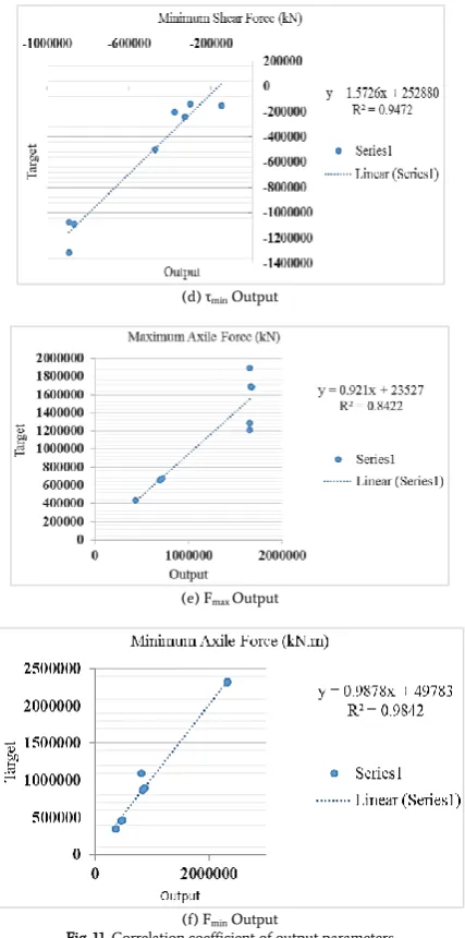
Where, var represents the variance, and are the kth measured and predicted values respectively, is the mean of predicted values, and N is the number of data sets. The VAF index express the intensity of variances discrepancy between the measured and predicted datasets. The values of VAF close to 100 % mean low inconsistencies, and therefore, better prediction capabilities. The lower RMSE, the better network’s performance [51, 52]. In an ideal condition, the RMSE value must be zero and the CE value must be 1.0. The graphs of R2 for output parameters are shown in Figs. 11(a)-(f).Table 4 presents the obtained values of performance indices.
(a) Mmax Output
(b) Mmin Output
(d) τmin Output
(e) Fmax Output
(f) Fmin Output
Fig. 11. Correlation coefficient of output parameters
Table 4. Performance indices of the model
Perform ance Index
Output parameters
M(Mome nt)max
M(Mome nt)min
τ(Shea r)max
τ(Shea r)min
F(Axia l)max
F(Axia l)min
RMSE
(%) 7 8 12 11 9 5
R2 0.962 0.95 0.92 0.95 0.84 0.98
VAF
(%) 94.21 94.36 91.54 89.3 88.9 98.4 CE 0.91 0.94 0.89 0.89 0.81 0.98
5.2.Sensitivity analysis
To determine the effect of each input parameter on output values, sensitivity analysis was performed. A useful method is cosine amplitude method (CAM) [53]. Data components form a data vector, X, are defined as:
x
1,
x
2,
x
3,...,
x
n
X
Every component xi in the data vector X, is a vector with m dimension, i.e.,
i1 i2 i3 im
i
x
,
x
,
x
,...,
x
x
Hence, all data can be assumed as a point in m-dimensional space, where each point has m coordinates for a full description. Each element of a relation, rij, results from a mutual comparison of two data pairs, i.e. xi and xj. The strength of the relationship between vector xi and vector xj is defined by Eq. (6):
m
k jk m
k ik m
k jk ik
ij
x x
x x r
1 2
1 2
1 (6)
Where, rij is strength of relations between input and output parameters, and i, j =1, 2, …, n. Eq. (6) defines that this method is the dot product of the cosine function. When two vectors are collinear (most similar), dot product will be unity; when orientation of 2 vectors have 90◦ of angle with respect to each other (most dissimilar), dot product will be zero.
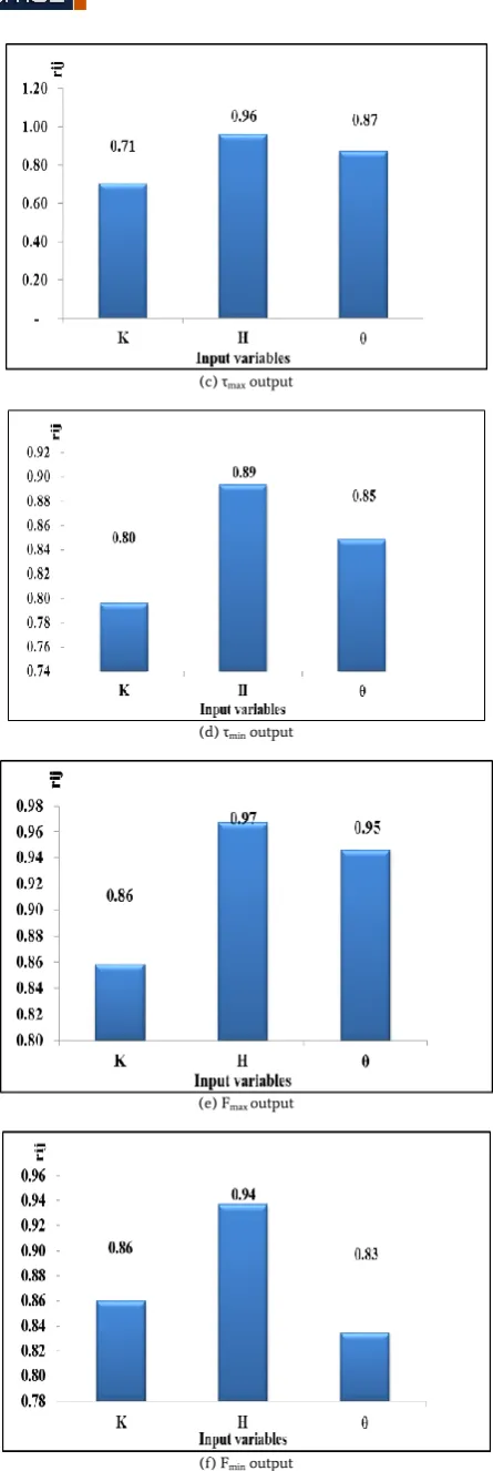
Figs. 12(a)-(f) show the strength values of relations (rij) between input (H, K, θ) and output parameters.
As can be seen from the Figs. 11(a)-(f), the overburden of buried tunnel or Height (H) input variable is the most efficient parameter on the resulted outputs than the other parameters two, and K value (lateral earth pressure) has the least influence on outputs except for Mmin and Fmin outputs.
(a) Mmax output
A. Rastbood et al. / Int. J. Min. & Geo-Eng. (IJMGE), 51-1 (2017) 71-78 77
(c) τmax output
(d) τmin output
(e) Fmax output
(f) Fmin output
Fig. 12. Strength of relation (rij) between input and output parameters
6.
Conclusion
The peak values of structural forces were determined for the structure of segmental tunnel lining ring using the ANN method. Neural network model of multi-layer perceptron was applied. At first, based on the minimum obtained values of RMSE from the input data variables, the number of neurons and their arrangement in hidden layers were determined and optimized. It was concluded that in 3-4-2-1 arrangement of neurons in the network, the resulted value of RMSE was 0.01 both for LOGSIG and TANSIG transfer functions. Then the NN model was tested and validated using different data. The efficiency of presented NN model was evaluated using the RMSE, R2, VAF and CE indices. The obtained results presented the high capability of the NN model in prediction and estimation of structural forces in segmental lining of tunnel, and this prediction method can be employed to gain reliable results for primary design of segmental tunnel lining instead of current tedious and expensive methods.
Finally, the sensitivity analyses were conducted to evaluate the effect of each input variable on the output parameters. It was found that the tunnel height or overburden parameter (H), among other input variables, had the highest influence on outputs, and the K parameter (lateral earth pressure) had the least effect on outputs. The reason is that the tunnel height is the main source of induced stresses on tunnel lining. On the other hand, other input variables, i.e. the lateral earth pressure and key segment position had the second order of importance on induced stresses than the tunnel height value.
References
[1] Arnau, O., & Molins, C. (2011). Experimental and analytical study of the structural response of segmental tunnel linings based on an in situ loading test. Part 2: Numerical simulation. Tunnelling and Underground Space Technology, 26(6), 778-788.
[2] Arnau, O., & Molins, C. (2012). Three dimensional structural response of segmental tunnel linings. Engineering Structures, 44, 210-221.
[3] Augarde, C., & Burd, H. (2001). Three‐dimensional finite element analysis of lined tunnels. International Journal for Numerical and Analytical Methods in Geomechanics, 25(3), 243-262.
[4] Beiki, M., Majdi, A., & Givshad, A. D. (2013). Application of genetic programming to predict the uniaxial compressive strength and elastic modulus of carbonate rocks. International Journal of Rock Mechanics and Mining Sciences, 63, 159-169.
[5] Benardos, A., & Kaliampakos, D. (2004). Modelling TBM performance with artificial neural networks. Tunnelling and Underground Space Technology, 19(6), 597-605.
[6] Bilotta, E., & Russo, G. (2013). Internal forces arising in the segmental lining of an earth pressure balance-bored tunnel. Journal of Geotechnical and Geoenvironmental Engineering, 139(10), 1765-1780.
[7] Chen, J., & Mo, H. (2009). Numerical study on crack problems in segments of shield tunnel using finite element method. Tunnelling and Underground Space Technology, 24(1), 91-102.
[8] Cybenko, G. (1989). Approximation by superpositions of a sigmoidal function. Mathematics of control, signals and systems, 2(4), 303-314.
[9] Den Hartog, M., Babuška, R., Deketh, H., Grima, M. A., Verhoef, P., & Verbruggen, H. B. (1997). Knowledge-based fuzzy model for performance prediction of a rock-cutting trencher. International Journal of Approximate Reasoning, 16(1), 43-66.
[10] Do, N.-A., Dias, D., Oreste, P., & Djeran-Maigre, I. (2015). 2D numerical investigation of segmental tunnel lining under seismic loading. Soil Dynamics and Earthquake Engineering, 72, 66-76.
[12] Einstein, H. H., & Schwartz, C. W. (1979). Simplified analysis for tunnel supports. Journal of Geotechnical and Geoenvironmental Engineering, 105(ASCE 14541).
[13] El Naggar, H., & Hinchberger, S. D. (2008). An analytical solution for jointed tunnel linings in elastic soil or rock. Canadian Geotechnical Journal, 45(11), 1572-1593.
[14] El Naggar, H., Hinchberger, S. D., & Lo, K. (2008). A closed-form solution for composite tunnel linings in a homogeneous infinite isotropic elastic medium. Canadian Geotechnical Journal, 45(2), 266-287.
[15] Etzkorn, B. (2011). Data Normalization and Standardization. Retrieved from http://www.benetzkorn.com/2011/11/data-normalization-and-standardization/ [16] Fausett, L. (1994). Fundamentals of neural networks: architectures, algorithms, and applications: Prentice-Hall, Inc.
[17] Flood, I., & Kartam, N. (1994). Neural networks in civil engineering. I: Principles and understanding. Journal of computing in civil engineering, 8(2), 131-148.
[18] Gajewski, J., & Jonak, J. (2006). Utilisation of neural networks to identify the status of the cutting tool point. Tunnelling and Underground Space Technology, 21(2), 180-184.
[19] Grima, M. A. (2000). Neuro-fuzzy modeling in engineering geology. AA Balkema, Rotterdam, 244.
[20] Habibagahi, G., & Katebi, S. (1996). Rock mass classification using fuzzy sets. [21] Hefny, A. M., & Chua, H.-C. (2006). An investigation into the behaviour of jointed tunnel lining. Tunnelling and Underground Space Technology, 21(3), 428. [22] Japan Society of Civil Engineers. (1996). Japanese Standard for Shield Tunnelling. Tokyo,Japan: JSCE.
[23] Kim, C. Y., Bae, G., Hong, S., Park, C., Moon, H., & Shin, H. (2001). Neural network based prediction of ground surface settlements due to tunnelling. Computers and Geotechnics, 28(6), 517-547.
[24] Koyoma, Y., & Nishimura, T. (1998). The design of lining segment of shield tunnel using a beam-spring model. Railway Technical Research Institute, Quarterly Reports, 39(1).
[25] Lawrence, J. (1993). Introduction to neural networks.
[26] Lee, K., & Ge, X. (2001). The equivalence of a jointed shield-driven tunnel lining to a continuous ring structure. Canadian Geotechnical Journal, 38(3), 461-483.
[27] Leu, S.-S., Chen, C.-N., & Chang, S.-L. (2001). Data mining for tunnel support stability: neural network approach. Automation in Construction, 10(4), 429-441. [28] Majdi, A., Ajamzadeh, H., & Emad, K. (2010). Numerical evaluation of the influence of bolted-and non-bolted joints on segmental tunnel lining behavior in line 4 Tehran subways. Paper presented at the ISRM International Symposium-6th Asian Rock Mechanics Symposium.
[29] Majdi, A., & Beiki, M. (2010). Evolving neural network using a genetic algorithm for predicting the deformation modulus of rock masses. International Journal of Rock Mechanics and Mining Sciences, 47(2), 246-253.
[30] Majdi, A., & Rezaei, M. (2013). Application of Artificial Neural Networks for Predicting the Height of Destressed Zone Above the Mined Panel in Longwall Coal Mining. Paper presented at the 47th US Rock Mechanics/Geomechanics Symposium.
[31] Majdi, A., & Rezaei, M. (2013). Prediction of unconfined compressive strength of rock surrounding a roadway using artificial neural network. Neural Computing and Applications, 23(2), 381-389.
[32] Majdi, A. a. A., M. (2007). Prediction of triaxial compressive strength of intact rock samples by artificial neural network. Paper presented at the Geotechnical Conference, Ottawa, Canada,.
[33] Mashimo, H., & Ishimura, T. (2003). Evaluation of the load on shield tunnel lining in gravel. Tunnelling and Underground Space Technology, 18(2), 233-241. [34] Molins, C., & Arnau, O. (2011). Experimental and analytical study of the
structural response of segmental tunnel linings based on an in situ loading test.: Part 1: Test configuration and execution. Tunnelling and Underground Space Technology, 26(6), 764-777.
[35] Morgan, H. (1961). A contribution to the analysis of stress in a circular tunnel. Geotechnique, 11(1), 37-46.
[36] O'Carroll, J. B. (2005). A Guide to Planning, Constructing, and Supervising Earth Pressure Balance TBM Tunneling: Parsons Brinckerhoff.
[37] Penzien, J., & Wu, C. L. (1998). Stresses in linings of bored tunnels. Earthquake engineering & structural dynamics, 27(3), 283-300.
[38] Ranken, R. E., Ghaboussi, J., & Hendron Jr, A. (1978). Analysis of ground-liner interaction for tunnels. Retrieved from
[39] Rezaei, M., Majdi, A., & Monjezi, M. (2014). An intelligent approach to predict unconfined compressive strength of rock surrounding access tunnels in longwall coal mining. Neural Computing and Applications, 24(1), 233-241.
[40] Rojas, R. (2013). Neural networks: a systematic introduction: Springer Science & Business Media.
[41] Rosenblatt, F. (1958). The perceptron: a probabilistic model for information storage and organization in the brain. Psychological review, 65(6), 386. [42] Rumelhart, D. E., Hinton, G. E., & Williams, R. J. (1988). Learning representations by back-propagating errors. Cognitive modeling, 5(3), 1. [43] Salemi, A., Esmaeili, M., & Sereshki, F. (2015). Normal and shear resistance of longitudinal contact surfaces of segmental tunnel linings. International Journal of Rock Mechanics and Mining Sciences, 77, 328-338.
[44] Santos, O. J., & Celestino, T. B. (2008). Artificial neural networks analysis of Sao Paulo subway tunnel settlement data. Tunnelling and Underground Space Technology, 23(5), 481-491.
[45] Shi, B. H., & Li, W. Q. (2012). Online Fault Prediction for EPB Shield Tunneling Based on Neural Network. Paper presented at the Advanced Materials Research.
[46] Teachavorasinskun, S., & Chub-Uppakarn, T. (2008). Experimental verification of joint effects on segmental tunnel lining. Electronic Journal of Geotechnical Engineering, 14, 1-8.
[47] Teachavorasinskun, S., & Chub-uppakarn, T. (2010). Influence of segmental joints on tunnel lining. Tunnelling and Underground Space Technology, 25(4), 490-494.
[48] Tiryaki, B. (2008). Application of artificial neural networks for predicting the cuttability of rocks by drag tools. Tunnelling and Underground Space Technology, 23(3), 273-280.
[49] Wittke, W., Erichsen, C., & Gattermann, J. (2006). Stability Analysis and Design for Mechanized Tunnelling. WBI, Felsbau GmbH, Aachen.
[50] Wood, A. M. (1975). The circular tunnel in elastic ground. Geotechnique, 25(1), 115-127.
[51] Working-Group, I. (2000). Guidelines for the design of shield tunnel lining. Tunnelling and Underground Space Technology, 15(3), 303-331.
[52] Ye, F., Gou, C.-f., Sun, H.-d., Liu, Y.-p., Xia, Y.-x., & Zhou, Z. (2014). Model test study on effective ratio of segment transverse bending rigidity of shield tunnel. Tunnelling and Underground Space Technology, 41, 193-205. doi:http://dx.doi.org/10.1016/j.tust.2013.12.011
[53] Zixin, Z., Yongsheng, L., & Xiaomin, Y. (2007). An analytical solution of shield tunnel based on force method Underground Space ? The 4th Dimension of Metropolises, Three Volume Set +CD-ROM: CRC Press.