University of Colorado Boulder, Boulder, CO 80309, USA
2Department of Aerospace Engineering, University of Illinois Urbana-Champaign, Champaign, IL 61820, USA 3Department of Mechanical Engineering, University of Texas at Dallas, Richardson, TX 75080, USA
4Department of Electrical Engineering, Colorado School of Mines, Golden, CO 80401, USA 5National Wind Technology Center, National Renewable Energy Laboratory, Golden, CO 80401, USA
6Department of Mechanical and Aerospace Engineering, University of Virginia, Charlottesville, VA 22904, USA
Correspondence:Daniel S. Zalkind ([email protected])
Received: 4 January 2019 – Discussion started: 6 February 2019
Revised: 2 August 2019 – Accepted: 26 September 2019 – Published: 11 November 2019
Abstract. We examine the effect of rotor design choices on the power capture and structural loading of each major wind turbine component. A harmonic model for structural loading is derived from simulations using the National Renewable Energy Laboratory (NREL) aeroelastic code FAST to reduce computational expense while evaluating design trade-offs for rotors with radii greater than 100 m. Design studies are performed, which focus on blade aerodynamic and structural parameters as well as different hub configurations and nacelle placements atop the tower. The effects of tower design and closed-loop control are also analyzed. Design loads are calculated according to the IEC design standards and used to create a mapping from the harmonic model of the loads and quantify the uncertainty of the transformation.
Our design studies highlight both industry trends and innovative designs: we progress from a conventional, upwind, three-bladed rotor to a rotor with longer, more slender blades that is downwind and two-bladed. For a 13 MW design, we show that increasing the blade length by 25 m, while decreasing the induction factor of the rotor, increases annual energy capture by 11 % while constraining peak blade loads. A downwind, two-bladed rotor design is analyzed, with a focus on its ability to reduce peak blade loads by 10 % per 5◦of cone angle and also reduce total blade mass. However, when compared to conventional, three-bladed, upwind designs, the peak main-bearing load of the upscaled, downwind, two-bladed rotor is increased by 280 %. Optimized teeter configurations and individual pitch control can reduce non-rotating damage equivalent loads by 45 % and 22 %, respectively, compared with fixed-hub designs.
Copyright statement. Christopher J. Bay’s copyright for this publication is transferred to Alliance for Sustainable Energy, LLC.
1 Introduction
Wind turbines are large, dynamic structures that experience significant structural loading on their component parts. De-sign choices impact the loading on each of these parts. We present a model for the rapid computation of wind turbine
COE=CapEx+OpEx
AEP , (1)
where capital expenditures (CapEx) and operational expen-ditures (OpEx) make up the cost of building and running a wind turbine. Our goal is to minimize the cost of wind en-ergy, enabling the sale of more wind turbines in an effort to make low-cost energy more available.
Operational expenditures are non-negligible but make up roughly 15 % of the total cost, according to a study of the av-erage 2015 offshore wind turbine (Mone et al., 2015). Capi-tal expenditures include the wind turbine parts and balance-of-station costs. Balance-balance-of-station costs account for about 55 % of the total cost and include electrical infrastructure, assembly, and substructure costs. Wind turbine parts (tower, nacelle, blades, etc.) comprise about 30 % of the overall cost of an offshore, fixed-bottom wind plant (Mone et al., 2015). The small cost contribution of the wind turbine blades, which is only a fraction of the cost of the wind turbine parts, and the significant effect of wind turbine blades on AEP contribute to the economics that enable larger and larger blades.
However, longer blades require additional structural re-inforcement, which increases the blade weight, resulting in larger loads experienced by other wind turbine components like the hub, main bearing, yaw bearing, and tower. Various innovations have enabled lower weight blades; these inno-vations are then used to subsequently design larger blades that capture more power. Still, the wind turbine components must survive extreme structural loading and last 20–30 years. Wind turbine components are often designed by various en-gineering teams based on loads from aeroelastic simulations, making wind turbine design a large, distributed design task.
The aerodynamic and structural aspects of wind turbines must be designed and controlled so that the structural load-ing for a design is feasible. There is a large interdependence between these design aspects (aerodynamic, structural, and controls) and on the various wind turbine components, which has led to numerous design optimization studies. These stud-ies focus primarily on blade aerodynamic and structural de-sign, e.g., in Ning et al. (2014) and Pavese et al. (2017). Some incorporate dynamic control effects, like Tibaldi et al. (2015) and Bortolotti et al. (2016). System engineering tools, like HAWTOpt2 (Døssing, 2011), WISDEM (Dykes et al., 2014), and Cp-Max (Bortolotti et al., 2016), have been developed to handle the large number of design variables but often com-pute structural loads using simplified scaling rules, conserva-tive static calculations, or many nonlinear aeroelastic simu-lations. A full set of design load cases (DLCs), specified by the International Electrotechnical Commission (2005) (IEC) in design standards, and simplified for research purposes in Natarajan et al. (2016), can include up to 2000 simulations, which can be costly in terms of computational effort, result-ing in long design cycle times. Often the results of these sim-ulations do not fully elucidate the root cause of problematic load cases on the affected turbine component. An attempt
to distill the DLCs into a reduced basis for design loads in an optimization framework was presented in Pavese et al. (2016).
We describe an alternative load estimation procedure, based on a set of simulations with a constant, sheared wind inflow that reflects the main drivers of wind turbine loads and the effects of design changes on global wind turbine loads. Since both turbulent and constant wind effects contribute to structural loading and the effect of turbulence has been well studied recently, e.g., in Dimitrov et al. (2018) and Robertson et al. (2018), we will focus our effort on how turbine model changes impact the harmonic loads caused by wind shear and turbine self-weight. We do this by decomposing the turbine loads from constant, sheared wind inputs into their harmonic components, i.e., the load amplitude of theith per revolu-tion (iP) load signal. These signals have been used for control (Bottasso et al., 2013), stability analysis (Bottasso and Cac-ciola, 2015), and wind field estimation (Bertelè et al., 2017). Here, we use the same signals to develop a mapping, or trans-formation, from the harmonic loads to the DLC-simulated design loads to understand the effect that changing the un-derlying turbine model has on structural loading.
The power and load estimation procedure developed in this study is used to analyze concepts for enabling rotor radii greater than 100 m. Recently, large rotor concepts have been studied in the European projects UpWind and INNWIND. The Danish Technical University (DTU) 10 MW reference wind turbine (RWT) (Bak et al., 2013) was provided as a design basis for large rotors to test design methods and tools. The DTU 10 MW RWT has motivated studies that fo-cus on optimization methods (Zahle et al., 2015) and active (McWilliam et al., 2018) and passive (Pavese et al., 2017) load control methods, but the resulting designs from these studies do not deviate far from the base rotor model. A two-bladed, downwind, teetering hub configuration of the DTU 10 MW RWT was developed, which shows that a teetering hub can greatly reduce the unbalanced loading on the main shaft and blade root (Bergami et al., 2014). Bergami et al. (2014) suggest that the tower stiffness distribution needs to be redesigned in order to avoid a resonance at the twice-per-revolution (2P) rotor harmonic and that two-bladed rotors (without teeter) increase loading on the main shaft signifi-cantly.
A couple of 20 MW rotor designs have been proposed in the literature. Sieros et al. (2012) and Peeringa et al. (2011) use classical similarity scaling rules to upscale conventional turbines. Both conclude that loads due to self-weight will in-crease significantly with blade length and drive component design as turbines grow larger. Specifically, edgewise blade loads and the effect of wind shear are magnified for larger rotor sizes.
the effects of significant design changes and detailed ro-tor upscaling on the various wind turbine components. We will quantify the effect of aerodynamic changes, including the blade length, axial induction, cone angle, and number of blades, as applied to both upwind and downwind rotors. A simplified structural model will demonstrate the effect of structural reinforcement on blade mass and loads. The upscaled structural model must provide enough stiffness to compensate for the increasing edgewise blade loads of large rotors. We quantify the effect of changes to the hub by look-ing at three-bladed and two-bladed rotor configurations, and consider the relative benefits of a teeter hinge or individual pitch control for the latter. Finally, we show how the nacelle placement atop the tower and control schemes can impact the loads on the tower and yaw bearing.
We believe this study will contribute an early stage de-sign model for evaluating dede-sign concepts with less compu-tational effort by eliminating hundreds of DLC simulations. The simplified load model provides a qualitative understand-ing of the relationship between wind turbine structural loads as they progress from the blades to the substructure, high-lighting the wind speeds where peak and fatigue loads are most problematic. A designer could use the simplified model to explore the design space and develop an initial wind tur-bine model for use in a more detailed load analysis. We map the harmonic loads to a set of loads found using operational design load case simulations and quantify the uncertainty. Quantitative design studies evaluate the effect of increased blade size and power capture on global wind turbine loads, as well as the design trade-offs associated with two-bladed wind turbines, teeter hinges, and individual pitch control.
We will present the baseline models used for compari-son and our general design direction in Sect. 2. Section 3 will outline the tools used for design and simulation and will also provide environmental site specifics. A description of the control scheme used throughout the article is pre-sented in Sect. 4. The harmonic model is described in Sect. 5, and in Sect. 6 the transformation from harmonic loads to DLC-simulated design loads is described. The set of design studies is described in Sect. 7, leading to studies of blade loads and power capture (Sect. 8), hub and main-bearing
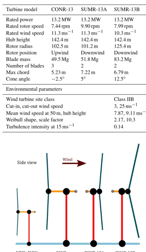
mination of a series of design studies aimed at designing a lightweight 100 m blade; it utilizes flatback airfoils, carbon-fiber reinforcement, and advanced core materials to reduce the blade mass below state-of-the-art scaling trends. The full design is described in Griffith and Richards (2014). The dis-tributed blade structural properties of the CONR-13 will be used for all three-bladed rotors in this study.
A downwind, two-bladed rotor was developed with simi-lar structural advances but with the goal of reducing the total blade mass by at least 25 % compared to the CONR-13 (Grif-fith, 2017). The blade was designed to enable segmentation, ultralight design, and a morphing rotor; we refer to this de-sign as the SUMR-13A. The initial aerodynamic dede-sign is presented in Ananda et al. (2018). We have slightly modified the initial design to have a downwind cone angle of 5◦ for the purposes of the design studies presented later. The dis-tributed structural parameters of the SUMR-13A blade were used as a basis for scaling all two-bladed rotors in this study. A summary of both baseline models is shown in Table 1 and are drawn to scale in Fig. 1. Both rotors were structurally validated to check strain limits, panel buckling, flutter, and fatigue.
In the remainder of this paper, we will evaluate designs aimed at
1. increasing the energy capture and
2. reducing the wind turbine component loads.
Table 1. Turbine models and environmental parameters used throughout this article.
Turbine model CONR-13 SUMR-13A SUMR-13B
Rated power 13.2 MW 13.2 MW 13.2 MW Rated rotor speed 7.44 rpm 9.90 rpm 7.99 rpm Rated wind speed 11.3 ms−1 11.3 ms−1 10.3 ms−1 Hub height 142.4 m 142.4 m 142.4 m Rotor radius 102.5 m 101.2 m 125.4 m Rotor position Upwind Downwind Downwind Blade mass 49.5 Mg 51.8 Mg 83.2 Mg Number of blades 3 2 2 Max chord 5.23 m 7.22 m 6.79 m Cone angle −2.5◦ 5◦ 12.5◦ Environmental parameters
Wind turbine site class Class IIB Cut-in, cut-out wind speed 3, 25 ms−1 Mean wind speed at 50 m, hub height 7.87, 9.11 ms−1 Weibull shape, scale factor 2.17, 10.3 Turbulence intensity at 15 ms−1 0.14
Figure 1.Illustrations of the turbines in this study, along with the National Renewable Energy Laboratory (NREL) 5 MW reference turbine (Jonkman et al., 2009) for comparison. Tower heights, rotor radii, and cone angles are drawn to scale; overhangs and nacelle center of masses are enlarged for comparison.
3 Design and simulation tools, wind turbine environment
Aerodynamic design was performed using two inverse de-sign tools: PROPID and PROFOIL. PROPID (Selig and Tan-gler, 1995; Selig, 1995) is an inverse rotor design tool that enables a rotor geometry to be designed based on desired per-formance specifications like available power, tip speed ratio, wind speed distribution, axial induction, airfoils used, and desired lift distribution along the blade. PROFOIL (Drela and Giles, 1987) is an inverse airfoil design tool. It allows for
the design of airfoil geometries based on prescribed velocity distributions and desired geometric (thickness and camber) and aerodynamic properties. Airfoil geometries output using PROFOIL are analyzed using XFOIL (Drela, 1989) and it-erated on using PROFOIL until a final converged design is obtained.
Aeroelastic simulations were performed using the latest version of FAST (Jonkman, 2013). Different FAST mod-ules couple the wind inflow with aerodynamic and elas-tic solvers that compute the structural loading on the wind turbine. Turbulent wind inputs are generated using Turb-Sim (Jonkman and Kilcher, 2012). A recent FAST-based, wind-tunnel-validated approach has shown that, compared with turbulence, tower shadow effects are relatively small (Noyes et al., 2018). Thus, for simplicity, we have omitted the tower shadow model from our analysis in order to fo-cus on the influence of the more important harmonic and tur-bulent loads. Control inputs are provided to FAST through a Matlab/Simulink interface that processes FAST outputs and performs closed-loop control. Fatigue results are com-puted using MLife (Hayman, 2012), which uses a rain-flow-counting algorithm to determine load cycles and extrapolates them over the lifetime of the wind turbine.
To properly compute lifetime fatigue and annual energy production, the wind turbine environment must be provided. The rotors in this study are all designed to be placed off the coast of Virginia, USA. The site corresponds to a Class IIB turbine rating (International Electrotechnical Commission, 2005), with mean and turbulent wind speed characteristics shown in Table 1.
4 Closed-loop control
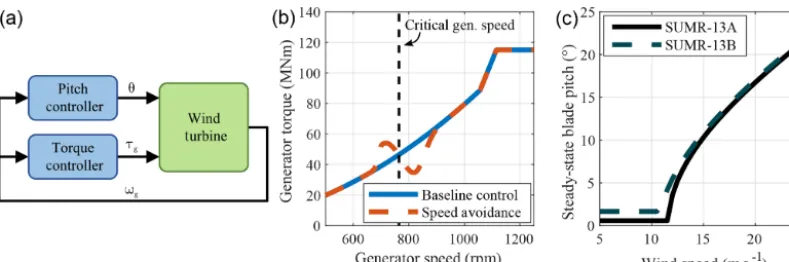
To simulate turbine design loads and power capture, a closed-loop control scheme is necessary. In below-rated conditions, the generator torqueτgis controlled so that the rotor speedω is optimal for power capture, following the typicalτg=kω2 law for most of the below-rated operating region, before tran-sitioning to above-rated conditions (Pao and Johnson, 2011). For simplicity, this is implemented as a look-up table, though more sophisticated methods exist. The look-up table is al-tered to avoid a critical rotor speed for two-bladed rotors only (see Fig. 2b; Sect. 11 provides more details). The generator rated power of 13.2 MW and rated speed of 1173.7 rpm are assumed to be constant for all the turbines in this study. The gearbox ratio of each turbine is changed to enable operation at the aerodynamically optimal rated rotor speed.
blade pitch angles(c)for the SUMR-13A and SUMR-13B.
many rotors in the same way. The optimal generator torque control gain kis computed using rotor parameters, and the PI pitch control gains are tuned using a subset of the DLC 1.2 turbulent simulations. The control architecture (as shown in Fig. 2a) is adapted from the National Renewable Energy Lab-oratory (NREL) 5 MW baseline controller (Jonkman et al., 2009), which is commonly used as a reference to compare new controller designs. While this baseline control may not necessarily be the best possible controller, it allows us to fo-cus on the power and load sensitivity to model changes.
Using closed-loop control for load simulations is impor-tant because peak loads often occur near the transition be-tween below- and above-rated operation. With a constant generator rating (13.2 MW), different rotors transition from below- to above-rated conditions at different wind speeds. Additional control signals, like individual pitch control (IPC) signals, are added to the baseline control signals in Fig. 2a.
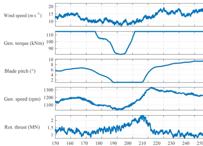
A controller is also necessary for computing design loads in turbulent DLC simulations, where wind speed changes, or gusts, must be adequately controlled. Often, peak loads are caused by a negative gust, or lull, which we show in Fig. 3. During a decrease in wind speed, the rotor slows and the pitch decreases to its optimal power position. When the de-crease in wind speed is followed by a positive gust, the pitch control must react quickly to regulate rotor speed. We model the actuator of each rotor in this study as a second-order But-terworth filter with a cut-off frequency of 0.25 Hz. The pitch actuator has a maximum pitch rate limit of 4◦s−1; maximum pitch rates between 1 and 3◦s−1 were recorded in the tur-bulent simulations that were run. This decrease and then in-crease in wind speed creates a condition where there is an above-rated wind speed but a below-rated pitch angle setting, resulting in a large thrust force on the rotor and high loads. To capture the effect that closed-loop control has on design loads as rotor changes are made, we use the same control architecture for computing loads using the harmonic model (Sect. 5) and for turbulent DLC simulations (Sect. 6), updat-ing the controller parameters based on the rotor parameters.
5 Harmonic model for load estimation
Load simulations according to the DLCs can be time con-suming, so we have developed a simplified model to esti-mate the loads on wind turbine components more quickly for evaluating design trade-offs across a wide range of parame-ters. In this section, we describe harmonic loadsmH, which are derived from constant and periodic loads that arise due to steady wind loading, wind shear, and turbine self-weight. These harmonic loads can be mapped, or transformed, into estimatesmEstof design loadsmDLCthat are computed using operational DLC simulations in Sect. 6. The key simplifica-tion of the harmonic load model compared to design loads computed using DLC simulations is the omission of load variations that occur at frequencies that do not correspond to the rotor speed. These non-harmonic load variations arise because of wind speed and direction changes, as well as the component’s natural frequencies. All frequency components of a load are required to determine the design load for a fi-nal, detailed design, but for exploring potentially large num-bers of design trade-offs, simplified harmonic loads provide enough information about the various turbine loads.
The harmonic loads are derived from FAST simulations with a sheared wind inflow such that the wind speedu at heightzis
u(z)=uh z
zh α
, (2)
wherezhis the hub height,uhis the wind speed at hub height, andα=0.14, which is representative of an offshore wind field (Jenkins et al., 2001). Because of the wind shear, the tur-bine’s structural load signals contain harmonic components that depend on the rotor azimuthψ; i.e., a load signalm(ψ) can be expressed as
m(ψ)=m0+m1Pc cos(ψ)+m1Ps sin(ψ)+. . .
Figure 3.Baseline control illustration of a problematic gust for the SUMR-13A baseline rotor in extreme turbulence (DLC 1.3) with a mean wind speed of 14 ms−1. The peak rotor thrust near 205 s causes the peak blade flapwise load for the SUMR-13A.
The components are computed by
m0= 1 2π NR
ψ
Z
ψ−2π NR
m(ψ)dψ, (4)
micP= 1 π NR
ψ
Z
ψ−2π NR
m(ψ) cos(iψ)dψ, (5)
and
misP= 1 π NR
ψ
Z
ψ−2π NR
m(ψ) sin(iψ)dψ, (6)
whereNRis the number of rotations used in the calculation (Phillips et al., 2007). We have found that load signals can be reconstructed closely using the first four harmonics; the most energy is usually in either the first, second, or third harmonic depending on the component (see Table 2) and number of blades.
From the components in Eqs. (5) and (6), the magnitude and phase of each harmonic can be computed:
m
iP =
q miP
c 2+
miP s
2
, (7)
and
φiP=tan−1 miP
s miP
c
. (8)
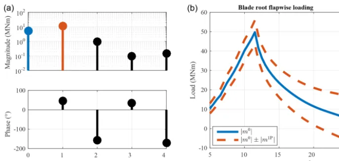
An example for the blade flapwise load is shown in Fig. 4; most of the load magnitude is in the constantm0and once-per-revolution m1P load component (101–102MNm), with some in the 2P load component due to shaft tilt and grav-ity (∼100MNm), and very little in the higher harmonics (<10−1MNm). We will use these harmonic coefficients, calculated via Eqs. (4)–(8), to estimate fatigue and extreme loads for the various wind turbine components.
5.1 Extreme and fatigue loads
The forces and moments on a component drive its design: larger loads require greater reinforcement, leading to greater component mass and cost. We analyze component loads in terms of the maximum (or peak) load:
mHPeak=maxu∈U
m0+mnP, (9)
wherenis the dominant harmonic signal component andUis the set of constant, sheared wind inputs used to derive the harmonic load. We perform simulations from in to cut-out (Table 1) in 0.5 ms−1increments.
Ta-Figure 4.Load harmonic magnitude|miP|and phaseφiP for the zeroth through fourth periodic harmonic of the blade root load in the flapwise direction(a)of the SUMR-13A at 25 ms−1. Mean load (blue) superimposed with the 1P harmonic amplitude (red) with respect to wind speed(b)used to estimate fatigue and extreme loads.
Table 2.Structural loads evaluated in this article. Each component has loads in multiple directions and experiences the peak load and greatest contribution to fatigue loads at different wind speeds.NBdenotes the number of blades on the rotor. Loads that are nearly constant across
wind speeds do not have a defined peak wind speed (N/A). The dominant wind speed contributing to fatigue is determined by analyzing the relative fatigue contribution,p(u)mnPfrom Eq. (10), across wind speeds.
Component Dominant Wöhler Load direction, Wind speed Dominant wind speed harmonic exponent name at peak load contributing to fatigue load
Blade 1P 10 Flapwise,mby Rated Rated Edgewise,mbx N/A Below rated
Hub 1P 3 Tilt,mhy N/A Rated
Yaw,mhz N/A Rated
Main bearing
NBP 3
Tilt,msy Rated/cut-out Rated (non-rotating) Yaw,msz Rated/cut-out rated
Yaw bearing NBP 3
Tilt,myy Rated/cut-out Rated Yaw,myz Rated/cut-out Rated
Tower NBP 3
Fore–aft,mty Rated Tower natural freq. Side to side,mtx Tower natural freq./cut-out Tower natural freq.
N/A indicates “not applicable”.
ble 1. We can relate the DEL of a component to its load har-monic by
mHDEL=aDEL(n, w) X
u∈U
p(u)mnP, (10)
where aDEL is a tuning factor that depends on the Wöhler exponentw and the dominant harmonic componentn. The dominant load harmonicnP of each component is either 1P orNBP, specified in Table 2, depending on whether the com-ponent is rotating (1P) or non-rotating (NBP). Different load harmonics will be specified by their location, direction, and harmonic number; e.g., the 3P main-bearing load about the ys axis will be writtenm3Psy. In this article, we focus on the moments about the load axes specified in Table 2 and illus-trated in Fig. 5. The loads at higher harmonic and natural
frequencies contribute to both fatigue and extreme loads, but since our goal is to derive a mapping from a simplified com-putation (harmonic load) to a more expensive simulation (de-sign load), their effects are neglected and considered as part of the uncertainty of the transformation in Sect. 6.
5.2 Harmonic versus turbulent loads
Figure 5.Illustration of the load axes used in this article. The non-rotating load axes – tower, main bearing, and yaw bearing – are all parallel and are denoted by subscripts “t”, “s”, and “y”, respectively. Note: the blade, hub, and main-bearing axis origins are collocated; the blade and hub load axes rotate with azimuth angle, as shown in Fig. 12. The CONR-13 is depicted to illustrate the rotor overhang xOHand nacelle center of massxcm. The prevailing wind is positive
in the same direction as thextaxis.
mapped to the design loads determined by the DLCs. We quantify this relationship in Sect. 6 by mapping the harmonic loads, computed using Eqs. (9) and (10), to the design loads computed in DLC simulations. In Sects. 7–11, we present the design load estimates and their uncertainties, transformed from harmonic loads, as various turbine design choices are evaluated.
6 Harmonic model transformation and uncertainty
To balance the computational efficiency of the harmonic load estimation in Sect. 5 with the more expensive and realistic design loads computed using DLC simulations, we present the following transformation procedure. In this article, we focus on the moments on the turbine components during power-producing design load cases and simulate the follow-ing DLCs specified by the IEC standard (International Elec-trotechnical Commission, 2005):
– DLC 1.2: normal turbulence, for fatigue loads, using six random seeds at mean wind speeds from cut-in to cut-out, spaced 2 ms−1apart.
– DLC 1.3: extreme turbulence, for peak loads, using the same number of turbulent wind seeds and wind speeds.
– DLC 1.4: extreme coherent gust with direction change, for peak loads near rated, above-, and below-rated wind conditions. Different rotor azimuthal initial conditions are simulated to account for the rotor being in different positions when the gust occurs.
– DLC 1.5: extreme wind shear, for peak loads near rated and at cut-out wind speeds. The same azimuthal initial conditions as in DLC 1.4 are used.
Fatigue loads are computed using the DLC 1.2 simulations in MLife (Hayman, 2012); they are extrapolated using the Weibull distribution in Table 1 to determine the lifetime DEL. The peak design load is determined using the maxi-mum (moment) over all the simulations in DLCs 1.3–1.5.
First, we compare the harmonic loads, calculated using the methods in Sect. 5, with the loads computed in DLC simula-tions. Then, we present a method to map the harmonic loads to the design loads, producing load estimates. Finally, we an-alyze the residual of the estimated loads, since not all rotors in the design studies of Sects. 7–11 will be simulated using the DLCs. Only a subset of the rotors analyzed in this article, indicated in Table 3, are used in the following procedure to transform the harmonic model. The design loads of a free-teetering hinge will not be included in the transformation set and uncertainty analysis for reasons described in Sect. 9.2; it is marked with an “x” in Fig. 6.
In Fig. 6a, we show the design load for the peak main-bearing load versus the harmonic load estimate. In general, the harmonic load estimate is much less than the design load computed in DLC simulations. For each component, part of the load can be attributed to the harmonic loading and part to the turbulent loading:
mDLC=mH+mturb. (11)
We quantify the turbulent load contribution mturb of each component load using the turbulence factor
fturb= mean m turb
mean mDLC (12)
to compare between different turbine parts on how much of the design loadmDLC is attributed to turbulent versus har-monic loading for Class IIB turbulence.
Figure 6.Peak main-bearing loads computed using DLC simulations versus the harmonic load(a)and transformed load estimates(b)for two-bladed rotors (cyan) and three-bladed rotors (magenta). The same color scheme is used to show the relative effect of turbulence on selected component loads(c), as defined in Eq. (12), and the standard deviation of the residual normalized by the mean load is shown for the whole transformation set(d). The loads presented in this study are specifically the moments about the specified axis.
Rotating component loads in turbulence are primarily driven by the 1P load, which is more clearly modeled by the har-monic loads, due to gravity and wind shear, than the smaller NBP load component.
We also see a difference in how turbulence affects two-versus three-bladed rotors, illustrated by the different lines of fit in Fig. 6a. In general, two-bladed rotors have a greater tur-bulent load component, but they also have a larger harmonic component, so the turbulence factor is similar to three-bladed rotors. For three-bladed rotors, the non-rotating load compo-nent DELs are not clearly modeled by their harmonic load, so they have a relatively high turbulence factor. Even though some turbine parts have large turbulent components that are not directly modeled by their harmonic loads, there is still good correlation between the harmonic and design loads.
We transform from the harmonic loads to the design loads by fitting a linear model,
mDLC=atransmH+btrans, (13)
and finding the linear least squares estimate of the param-etersatransandbtrans. Because two- and three-bladed rotors sample turbulence differently, we define a transformation set
(atrans,btrans) separately for each, illustrated by the different fits of Fig. 6a. There are also different transformation sets for each design load: at each axis and for both peak and fa-tigue loads. To estimate the design load, the transformation set corresponding to the desired component, axis, and num-ber of blades is used:
mEst=atransmH+btrans, (14)
which results in a transformed load estimate equal to the de-sign load, plus some residual (Fig. 6b).
We analyze the uncertainty of the transformation by com-puting the residuals between the estimated loads, which are fit using the linear relation (Eq. 14), and design loads of the set of rotors specified in Table 3. In Fig. 6d, we normalize the standard deviation of the residual by the mean load over all rotors to use a qualitative metric comparing the fit of the transformation across different turbine parts. We present the standard deviation of the residual without this normalization for each measure in the figures of Sects. 7–11.
DLC-Table 3.Set of turbines designed and analyzed in this article.a de-notes a turbine for which DLC simulations were performed and used to map the harmonic load estimates to DLC-based design loads. Otherwise, only the harmonic load analysis is performed.
b was omitted from the transformation set.cdenotes the
SUMR-13A rotor andddenotes a three-bladed variation of the SUMR-13A rotor. The process for using axial induction as an independent de-sign variable will be described in the rotor aerodynamic trade stud-ies section (Sect. 8.1).
Baseline set (Sect. 2): CONR-13a, SUMR-13Aa,c, SUMR-13Ba Rotor aerodynamic trade studies (two-bladed, Sect. 8.1): Available rotor power (MW): 13.9a,c, 14.9, 15.9, 16.9a
Axial induction (–): 0.175a, 0.200, 0.225, 0.250, 0.275, 0.300, 0.333a,c Cone angles (◦):−5a, 0, 5a,c, 10, 15, 20a
Rotor aerodynamic trade studies (three-bladed, Sect. 8.1): Available rotor power (MW): 13.9a,d, 14.9, 15.9, 16.9a
Axial induction (–): 0.175a, 0.200, 0.225, 0.250, 0.275, 0.300, 0.333a,d Cone angles (◦):−5a, 0, 5a,d, 10, 15, 20a
SUMR-13B structural parameter analysis (Sect. 8.2):
kAll=0a,kM=1,kFs=1,kEs=1,kAll=1a SUMR-13B hub configurations (Sect. 9): SUMR-13B (three-bladed)a
Teeter: freeb, ideala IPC: bladea, bearinga
computed design loads. The cases with lowest uncertainty tend to have lower turbulence factors, like the blade edge-wise (blade X) DEL and the hubzh-axis DEL. The AEP is also very well estimated by the harmonic model, which is good for power capture predictions as long as the effects of turbulence are transformed.
The most erroneous load component is the peak yaw-bearing load about the yyaxis, which has a large turbulent component and where a subset of the transformation set (the aerodynamic trade study designs) controls a problematic gust event, like the one in Fig. 3, similarly. These rotors have de-sign loads that are about the same for each, despite the differ-ences predicted by the harmonic model. The design loads for this component might be more a function of the gust event than the turbine configuration.
In the remainder of this article, we use these mapped load estimates to analyze the structural loading and power capture of the various rotor configurations in Table 3.
7 Overview of design studies
In this section, we outline the design and simulation results of the 42 turbines shown in Table 3. The design loads for each rotor are estimated using harmonic loads from Sect. 5 and the transformation method in Sect. 6. Additionally, gross AEP is calculated using the generator power P(u) at mean wind speeduby
AEP=8760X u∈U
p(u)P(u), (15)
wherep(u) is the Weibull distribution in Table 1 and 8760 is the number of hours in a year.
We first examine changes to the blade loads and power capture of the SUMR-13A due to variations in the aero-dynamics, including the blade length, axial induction, and cone angles. Both upwind (negative) and downwind (posi-tive) cone angles are evaluated. The aerodynamic changes lead to a larger, heavier but more powerful SUMR-13B ro-tor, which we use to study the effect of mass and stiffness scaling on blade loads. Next, non-rotating component loads will be compared for different hub configurations, consider-ing the number of blades, a teeterconsider-ing hconsider-inge, individual pitch control, and rotor placement (upwind versus downwind). Fi-nally, the effect of a downwind rotor on yaw-bearing design loads will be presented and the effect of a two-bladed rotor on tower design will be investigated. A summary of the de-sign parameters considered in this article and the process for incorporating their interconnections is shown in Fig. 7; de-tails are given in Sects. 8–11.
8 Blade loads and energy capture
We begin by analyzing the effect of changing rotor aerody-namics on blade loads and energy capture. Blade loads are computed at the blade root in both the flapwise (mby) and edgewise (mbx) directions. Blade flapwise loads are primar-ily aerodynamic in nature and depend on the thrust force ex-erted on the blades from the wind inflow. Peak blade flap-wise loads occur near rated wind speed, which represents the worst combination of wind speed and orthogonal blade surface area but before the blade begins pitching to regulate power in the above-rated operation. Blade pitch has a signif-icant influence on the mean blade flapwise load and control actions can often cause peak loads, e.g., when the pitch angle decreases towards its fine pitch angle to maximize power and then a wind speed gust occurs. The dependence of this load on the control system highlights the necessity of including control design at an early stage.
Figure 7.Overview of the design studies performed in this paper. The loads on each component (blue) transfer from the blades to the tower base as shown. Design studies (yellow) that affect each component are performed in Sects. 8–11 by altering the design parameters in green. Rotor design parameters (orange) affect all aspects of turbine design.
8.1 Rotor aerodynamics
We evaluate rotors with longer blade lengths, lower axial in-duction factors, and large, downwind cone angles, using the SUMR-13A design described in Sect. 2 as a baseline. These design studies have led us to an updated, larger, two-bladed design, indicative of the trends in industry towards longer, more slender blades but with a greater downwind cone an-gle. We will call this new rotor SUMR-13B (see Table 1 for more details).
Blade length is changed indirectly in PROPID by increas-ing the available rotor power at 11.3 ms−1 from 13.9 to 16.9 MW. However, all rotors are controlled to have the same rated generator power of 13.2 MW, which limits the increase in peak blade loads by transitioning to above-rated control
at lower wind speeds.1 The increased rotor-swept area in-creases both power capture and blade loads; a 10 % increase in rotor radius results in about a 10 % increase in AEP and 15 % increase in peak blade flapwise load (blue, left column in Fig. 8). For the blade length design study, the axial induc-tion factor along the outer three-fourths of the blade is fixed at13(theoretical Betz limit).
The rotors used to evaluate axial induction (red, center column in Fig. 8) are designed by fixing the flapwise root bending loads to that of the SUMR-13A and fixing the avail-able rotor power at rated wind speed to 13.9 MW. The blade length, chord, and twist are allowed to vary as the local axial induction factor – from the 25 % radial location to the blade
1The available rotor power of 13.9 MW at 11.3 ms−1and rated
Figure 8.Summary of aerodynamic design studies: the blade length, axial induction (in combination with blade length, chord, and twist), and cone angle are varied, while the AEP and peak blade load are calculated and compared to the base case (SUMR-13A, black dot in all). The standard deviations of the residuals for AEP and peak flapwise load are normalized to the SUMR-13A values and apply across all design studies. All rotors here are two-bladed, and positive cone angles correspond to downwind rotors. Unless otherwise specified, the available rotor power is 13.9 MW, the axial induction is 0.333, and the cone angle is 5◦.
tip – varies from 0.175 to 0.3 in increments of 0.025. De-creasing the designed axial induction of the rotor results in longer, more slender blades that capture more energy while constraining blade loads. In the most extreme example, a blade with a 0.175 axial induction factor can increase the AEP by 5 %, compared to a rotor with aerodynamically op-timal blades (axial induction factor of 13) but requires 16 % longer blades.
The cone angle design study is performed using the same baseline SUMR-13A blades for each rotor but with differ-ent cone angles, including upwind (negative) and downwind (positive) cone angles. With a fixed blade length, downwind, highly coned rotors decrease the rotor-swept area, resulting in both reduced power capture and blade loads. The load de-crease is significant: 25 % compared with a 7 % dede-crease in power capture. In comparison with the blade length design study, it is clear why highly coned rotors are attractive for large rotor designs: an increased cone angle will decrease operational loads faster than an increase in blade length will increase them.
For all the aerodynamic design studies, there is a trade-off between power capture and blade loading. Each design study is plotted together in Fig. 9, which also indicates the DELs in the flapwise and edgewise directions. In rotor design, our goal is to increase AEP and decrease blade loads, thus aiming to yield results in the lower right quadrant of each plot.
The SUMR-13A blade design was found to be driven by extreme loading along a combined flapwise and edgewise direction, where DLC 1.4 (extreme coherent gust with di-rection change) caused the greatest blade load. Since
edge-wise loads are largely deterministic, varying with a near-constant amplitude with respect to the rotor azimuth, the de-sign goal of the next rotor iteration, the SUMR-13B, was to constrain peak flapwise loads and increase power capture using the aerodynamic design changes previously described. The SUMR-13B is not necessarily cost optimal. Using larger blades with both greater power capture and structural load-ing could potentially result in a net cost benefit compared to the SUMR-13B. However, in the absence of a detailed cost model, these design choices are difficult to make and depend on a wide array of factors. Larger rotors with both increased loading and power capture will be investigated in future de-sign iterations.
Figure 9.The trade-off between power capture and blade loads. The AEP is plotted on thexaxis and blade loads are plotted on theyaxis. All rotors are normalized to the two-bladed 101.2 m SUMR-13A baseline rotor design (black dot). Each dot represents a rotor design and each curve represents the variation of one design parameter. The set of three-bladed rotor designs is represented with dotted curves. Unless otherwise specified, the available rotor power is 13.9 MW, the axial induction is 13, and the cone angle is 5◦; the SUMR-13B is specified in Table 1. The normalized residual standard deviation for AEP is the same as in Fig. 8, and the load residual standard deviations are normalized to the corresponding SUMR-13A values. The vectors indicate design changes in combination: blade length increase (blue diamond), axial induction factor decrease along with corresponding blade length increase (red, dashed vector), and cone angle increase (yellow, dashed vector) from the SUMR-13A to the SUMR-13B (square).
indicated by the dashed yellow vector. The combination of these design changes results in the AEP and structural load-ing of the SUMR-13B: it increases AEP by 11 % compared to the SUMR-13A while constraining peak blade flapwise loads to the level of the SUMR-13A. The same changes can be applied in combination to the flapwise DELs and edge-wise DELs. The increased blade length of the SUMR-13B increases the flapwise DELs due to the enhanced effect of wind shear and edgewise DELs due to the additional blade weight. During the SUMR-13B structural lay-up design, we found the design driving blade load to be the fatigue DEL in the edgewise direction, which will be the focus of Sect. 8.2.1. A set of three-bladed rotors (shown with dotted lines in Fig. 9) is designed similarly to the two-bladed design studies and exhibit similar trends to the two-bladed rotors in terms of blade loads. The blades of the three-bladed rotors experience lower loads (both peak and fatigue, edgewise and flapwise) with the same power capture due to their smaller chord and mass.
Despite the larger blade loads on two-bladed rotors com-pared to three-bladed rotors with the same power capture, we will be analyzing the two-bladed SUMR-13B for the re-mainder of this article. When comparing similarly powered rotors, e.g., the CONR-13 and the SUMR-13A, two-bladed rotors reduce the total blade mass by as much as 25 %, which reduces the capital expenditures associated with blade mate-rial costs (Griffith, 2017). Given the constant AEP and de-crease in CapEx of the two-bladed rotors, we would expect
the overall COE of a two-bladed rotor to be less than that of a similarly powered three-bladed rotor. However, periodic effects are more pronounced on the non-rotating components of two-bladed rotors. We will analyze the load-alleviating po-tential of different hub configurations in Sect. 9 and structural reinforcement in Sect. 8.2.
8.2 Blade structural parameters
To model blades with different lengths, we start with clas-sical similarity scaling rules (Loth et al., 2017a), based on the length scaling factor:
η=L/L0, (16)
whereLis the length of the scaled blade andL0is the length of the original blade. In this study, L0 is the length of the baseline blades: the SUMR-13A for two-bladed rotors and the CONR-13 for three-bladed rotors. We will examine the scaling of the following parameters (Griffith and Ashwill, 2011):
– mass per unit length, which scales withη2;
– stiffness per unit length in the flapwise, edgewise, and torsional directions, which scales withη4;
– stiffness per unit length in the spanwise direction, which scales withη2; and
– inertia per unit length in the flapwise and edgewise di-rections, which scales withη4.
Once integrated over the blade length, e.g., the mass scales with η3, while the stiffness and inertia properties scale withη5.
These parameters can be more flexibly scaled to account for innovations or changes to the structural design. For in-stance, we scale the mass per unit length distribution by
M(r)=M0(r)η2kM, (17)
whereM(r) is mass per unit length at spanwise locationr of the scaled blade, M0 is the mass per unit length of the original blade, andkM is a tunable parameter to increase or decrease the blade mass. Based on Eq. (17), once integrated over the blade length, kM=0 would produce a blade with a mass that scales linearly with blade length, whilekM=1 would produce a blade with a mass that scales with the cube of blade length. State-of-the-art trends show that mass scales roughly with the square of blade length, orkM=0.5. A sim-ilar parameter can be defined for stiffness scaling:
ks,flap=ks,flap,0η4kFs, (18)
whereks,flap is the flapwise stiffness per unit length of the scaled blade,ks,flap,0is the flapwise stiffness per unit length of the original blade, and kFs is a tunable flapwise stiffness scaling parameter. The edgewise stiffness will be similarly scaled using a parameter kEs. Flapwise and edgewise iner-tia is scaled using the same mass-scaling parameterkM but to the fourth power as in Eq. (18). Torsional and spanwise stiffness is scaled according to the similarity scaling rules defined above, withη4andη2, respectively. The SUMR-13B (two-bladed,η=1.24) structural properties are scaled from the SUMR-13A blade, first separately each for the mass and
stiffness parameters, and then all together (full scaling) in Fig. 10.
Ultimately, the final structural parameters will be deter-mined by the structural lay-up, but this model could be used to more quickly analyze trade-offs between blade mass, stiff-ness, loads, and power. In general, mass scaling has the great-est impact on loads. Since this article only considers op-erational load cases, the effect is most apparent when ana-lyzing fatigue loading. Loads during shutdown events and fault cases are also expected to increase with blade mass. Increased flapwise stiffness contributes to a small increase in energy capture (about 1 %; not shown) due to decreased blade deflection. We also observe that the change in load due to each individual scaling parameter (kM,kFs, andkEs) ap-proximately sum (or combine linearly), when multiple pa-rameters are simultaneously scaled. This is shown in Fig. 10: the sum of the changes in load due to mass, flap. stff., and edge stff. is approximately equal to the change in load due to full scaling. The same is true for the final design, which is a combination of the scaling parameters that are determined in the next section.
8.2.1 SelectingkMandkEsfor edgewise fatigue loads The most significant impact of positive structural scaling is the increase in edgewise DELs due to the increased blade mass. Theoretically, the additional mass increase of the larger blade would provide additional reinforcement against these loads, through trailing edge reinforcement or increased root diameter. We see that changes to the blade mass result in a change in edgewise loadδmbx, i.e.,
δmbx=a1kM+b1, (19)
wherea1andb1are determined from FAST simulations of the SUMR-13B blade with multiplekM values from 0 to 1 by finding the linear relationship betweenkMandδmbx. Ad-ditional edgewise stiffness must compensate for the increase in edgewise load by increasing the ultimate load:
mult= 2σEIx
c , (20)
where σ is the fiberglass strain limit at the trailing edge, EIx is the edgewise stiffness, andcis the blade chord; this is a simplification that assumes the neutral axis is at mid-chord (Budynas and Nisbett, 2015). In terms of the scaling coefficients, a linearized version of Eq. (20) can be obtained:
kEs=a2δmbx+b2. (21)
Finally, changes to the blade structural lay-up in the form of trailing edge reinforcement to increase edgewise stiffness will increase the blade mass:
The standard deviation of the residual is computed using the transformation set in Table 3 and is normalized to the non-scaled SUMR-13B.
Table 4.Blade structural coefficients for the SUMR-13B blade de-termined using the relationships described in Fig. 11.
Structural relations Final design coefficients
a1=0.51,b1=1.40 δmbx=1.8 a2=0.95,b2= −0.79 kEs=0.92 a3=0.87,b3=0 kM=0.804
Figure 11.The relationship between blade mass, edgewise loads, and edgewise stiffness, as well how each value was derived.
wherea3andb3are determined through a linear regression of SUMR-13B blade designs in NuMAD (Berg and Resor, 2012) with a targetkEsfrom 0 to 1. Additional trailing edge reinforcement was applied to meet the target values within 5 % and thekMwas computed using the overall mass of the resulting blade model.
The linear system determined by Eqs. (19), (21), and (22) can be solved to determine the necessary structural reinforce-ment for accommodating the load increase due to the in-crease in mass. See Table 4 for the results. These parame-ters can serve as targets for a detailed SUMR-13B structural lay-up design. For the remainder of this study, we will eval-uate the loading on other components as a result of the mass increase shown in Table 4.
9 Hub configuration and main-bearing loads
Blade loads are transferred through the blade root to the hub at the pitch actuator. In this section, we analyze the load cycle amplitudes of the hub loads and how they transfer to the non-rotating turbine components. The hub load axes,yh andzh, rotate with the hub (Fig. 12). About theyhaxis, hub loads are directly related to the blade loads for both two- and three-bladed configurations; they peak when the rotor is near ψ=0◦due to vertical wind shear, resulting in a large cosine– cyclic component of the hub load about theyhaxis (m1Phy,c). A teeter hinge reduces the coupling between blade and hub loads, except in cases of very large rotor deflections, where “hard” end stops increase the coupling and result in large peak loads. About thezhaxis, the source of loading depends on whether the rotor has two or three blades (see Fig. 12). For three-bladed rotors, the hub load about thezhaxis is driven by the blade aerodynamic loading due to wind shear and has a similar magnitude to the load about theyh axis (Fig. 12, top right). This symmetry is not inherent in a two-bladed configuration; themhz load is primarily determined by the weight of the blades unless there is a horizontal wind shear. The mismatch between the load cycle amplitudes ofmhyand
mhz results in larger non-rotating loads, e.g.,msy, for two-bladed rotors (Fig. 12, bottom right). The hub load about the zhaxis, for both hub configurations, peaks when the rotor is atψ=90◦, resulting in a largem1Phz,scomponent. The mag-nitude of these loads in relation to each other is important for determining their impact on the non-rotating load com-ponents.
The rotating hub is connected to the main shaft, which is supported by a main bearing close to the hub and also may consist of additional bearings between the hub and gearbox. A rotation matrix models the transfer of loads from the rotat-ing to non-rotatrotat-ing frame:
msy
msz
=
cosψ −sinψ sinψ cosψ
mhy
mhz
Figure 12.The hub axis (h) as it rotates with the rotor azimuth angleψfor a three- and two-bladed rotor. Note that theysaxis in Fig. 5 does
not rotate, while theyhaxis in Fig. 12 does. An example time series of the hub loads (mhyandmhz) is shown to demonstrate the difference in the non-rotating main-bearing load (msy) for a three-bladed (upper) and two-bladed (lower) SUMR-13B rotor.
which results in the 1P hub loads mapping to large 0P and 2P load components. The large 2P loads result in large fatigue DELs on the non-rotating parts of two-bladed turbines. The hub configuration, including the number of blades, whether a teeter hinge is used, and IPC all have an impact on the fatigue loading of the main bearing.
9.1 Number of blades
To compare with the two-bladed SUMR-13B, a three-bladed SUMR-13B was designed using the same blade parameters described in Table 4. Peak and fatigue blade loads in both the flapwise and edgewise directions are unaffected by the change in the number of blades.
Loads on other turbine parts are, however, affected by the change in the number of blades. Hub loads on the two-bladed SUMR-13B are mostly about theyhaxis (see m1Phy,c in Ta-ble 5), while three-bladed rotors are balanced in both direc-tions. The hub loads in Table 5 can be mapped to the non-rotating frame by Eq. (23). The 1P harmonic in the non-rotating frame transfers to 0P and 2P harmonics according to
m0Psy=1 2
m1Phy,c−m1Phz,s (24)
m2Psy=1 2
m1Phy,c+m1Phz,s. (25)
The 3P component is determined similarly based on the 2P harmonic load components by using Eq. (23).
Three-bladed rotors are advantageous due to these bal-anced hub loads, which effectively nullify the 2P load
com-ponents and only contain a small 3P load on the non-rotating turbine components. The difference in magnitude of the 1P hub load harmonics is responsible for the greater loading on the non-rotating components of two-bladed rotors. Fig-ure 13 shows more than a 20 % reduction in main-bearing DEL for the three-bladed SUMR-13B, compared to the two-bladed, fixed-hub SUMR-13B, even though the three-bladed rotor captures significantly more energy.
9.2 Teeter and individual pitch control
Historically, some two-bladed turbines have used a mechan-ical teeter hinge, which allows for rotation about an axis per-pendicular to the main shaft at the shaft tip. Recently, with the advent of pitch regulated turbines, individual pitch con-trollers have been designed in order to mimic this action by changing the aerodynamic loads on the blades as they ro-tate. Both solutions reduce loading on the hub, which trans-lates into reduced loading on the main bearing and other non-rotating components.
We have modeled a free-teetering hinge in FAST by en-abling the teeter degree-of-freedom and setting a zero damp-ing coefficient to the teeter motion. This free-teeterdamp-ing setup would provide the best configuration for reducing blade loads. A more realistic teeter hinge must account for friction, damping, and end stops (see, e.g., Schorbach et al., 2017).
Bearing IPC 17 700 −16 200
Three-bladed fixed hub SUMR-13A (3b) 7180 −7220 SUMR-13B (3b) 24 900 −24 700
Upwind rotors Two-bladed fixed hub SUMR-13A 3780 −3570 Three-bladed fixed hub SUMR-13A (3b) −526 543
Figure 13.Change in peak main-bearing loads(a)for the SUMR-13A cone angle study (two- and three-bladed rotors) and the SUMR-13B fixed-hub configuration, change in main-bearing DELs(b)about theysaxis (DELs about thezsaxis are within 5 % of theys-axis DELs)
and change in AEP(c)for various hub configurations of the SUMR-13B, compared with the fixed-hub, two-bladed SUMR-13B final design described in Sect. 8.2. The DEL and AEP results from different hub configurations(b, c)are design loads computed directly from DLC simulations.
and harmonic loads in Table 5 suggest that main-bearing fa-tigue loads (m2Psy) increase when compared to the fixed-hub configuration. However, DLC simulations show that turbu-lence has a relatively minimal impact on the non-rotating components for this rotor with a free-teetering hinge, com-pared with all other rotors. In other words, the design loads for the main bearing are nearly equal to the harmonic loads, but in every other case there is a significant turbulent compo-nent, as mentioned in Sect. 6. Since this case is an outlier and behaves differently when mapping harmonic loads to turbu-lent loads, it is omitted from the transformation set of two-bladed rotors. Instead of presenting the transformed load es-timates and power capture, we present the design loads com-puted directly from DLC simulations in Fig. 13. However,
the harmonic loads in Table 5 still illustrate how an optimal teeter design could mimic the balanced hub loads of three-bladed rotors.
A more ideal teeter design could be achieved by selecting an appropriate teeter damping coefficientdteet that matches them1Phy,c andm1Phz,s load harmonics to minimize the main-bearing loadm2Psy. Since only one damping coefficient must be designed for all wind speeds, we minimize the main-bearing load using the wind speed distributionp(u) by
dteet,opt=argmindteet X
u∈Uteet
p(u)m2Psy, (26)
greatest fatigue contribution occurs. Main-bearing load cy-cle amplitudes (m2Psy andm2Psz) increase with wind speed due to the increased effect of wind shear, but lower wind speeds are far more probable than high wind speeds. Since our de-sign goal is to reduce fatigue loads on the main bearing and other non-rotating components, we focus on below-rated wind conditions. The ideal teeter design greatly reduces the main-bearing fatigue loads, along with the fatigue loading on the other non-rotating components but reduces energy cap-ture by 1.9 %, compared with the fixed two-bladed SUMR-13B (Fig. 13b, c).
Alternatively, IPC can be used to mimic the rotor balanc-ing of a teeter hbalanc-inge by addbalanc-ing a time-varybalanc-ing pitch angle off-set to each blade. An IPC algorithm was initially designed to focus on blade loads, which we call blade IPC in Table 5 and Fig. 13. The two-bladed IPC architecture used here was ini-tially presented in van Solingen and van Wingerden (2015), which minimizes the teeter load:
mteet= 1
2 mby,1−mby,2
. (27)
We have applied loop-shaping procedures (McFarlane and Glover, 1992) to fine tune the controller to reduce the 1P and 2P blade harmonics, which results in a decrease in the blade design load for the SUMR-13B (about 10 % for flapwise peak and fatigue loads). The IPC algorithm was designed to operate in both above- and below-rated conditions, since the bulk of the fatigue loads occur in below-rated conditions, and the IPC must be active near rated in order to reduce the peak design load. Since this blade IPC is designed to reduce blade loads as much as possible, hub loads about theyhaxis are less than hub loads about thezh axis (Table 5). Therefore, the blade IPC algorithm is not necessarily optimal for the main-bearing DELs.
Using the relationship in Eq. (25), we designed a bear-ing IPC algorithm with the goal of balancbear-ing the hub load components, such thatm1Phy,c= −m1Phz,s, to minimize 2P load-ing on the main bearload-ing. Equivalently, m1Phy andm1Phz should be equal in magnitude and 90◦ out of phase. Since |m1Phz| changes more slowly than|m1Phy|, the mhz signal is delayed by 90◦and the difference,
md=mhy−mhz(ψ−90◦), (28)
can be fed back using the same architecture as the blade IPC becausemhy=2mteet. Harmonic load estimates suggest better load mitigation than those in Fig. 13, so we present the DLC-based design loads directly from turbulent simula-tions. In general, dynamic control solutions are not as well estimated using harmonic load estimates, compared with changes to the rotor model using the same control because dynamics due to turbulence often drive control design. Other control methods were attempted to balance the load compo-nents in Eq. (25), which are further explored in Zalkind and Pao (2019).
If used in below-rated conditions, these load mitigation techniques reduce power capture, as shown in Fig. 13c. IPC can be designed so that it only operates in above-rated con-ditions, resulting in a negligible power loss. However, this reduces its effectiveness in constraining peak loads that oc-cur close to rated wind speeds.
9.3 Large cone angle effects
The main bearing must support the weight of the rotor and thrust imbalance on the rotor due to shear, i.e.,
m0sy=m0sy,grav+m0sy,shr. (29)
For downwind turbines, both components of Eq. (29) are pos-itive, resulting in large, constant main-bearing loads about the ys axis. For upwind turbines, the load due to grav-ity m0sy,grav is negative, while the load due to wind shear m0sy,shr is positive, which greatly reduces the steady-state main-bearing load for upwind turbines compared to down-wind turbines. To quantify this difference, we analyze the harmonic load estimate of the peak main bearing (msy,Peak= m0Psy+m2Psy) for rotors with various cone angles (Fig. 13a).
The harmonic loads in Table 5 suggest there would be a significant change in the mean main-bearing loadm0Psy going from upwind to downwind rotor configurations. However, the design loads computed using DLC simulations show that turbulence contributes a large amount to the peak load expe-rienced by the main bearing (Fig. 6) for both configurations. A downwind configuration, compared to the same rotor up-wind (with cone angles of±5◦, respectively) only increases the main-bearing load by about 15 %. Despite the larger total blade mass of the three-bladed rotors, two-bladed rotors still have a larger peak load due to the increased 2P loading and a larger turbulent load component. We see this same effect in the fatigue loading results of Fig. 13, which suggests that peak main-bearing loads could be reduced using the same methods as in Sect. 9.2. The larger SUMR-13B, however, has a non-negligible increase in the peak main-bearing load, due to combined increases in blade mass, blade length, and cone angle. These increased loads on the main-bearing transfer to the other non-rotating components, which we will analyze in the yaw-bearing and tower design studies.
10 Yaw-bearing loads and nacelle layout
nacelle center of mass(b)required to balance the rotors, and the peak yaw-bearing loads(c)of the balanced rotors.
be counteracted by properly balancing the nacelle center of mass atop the tower. We will study the different cone angle designs from Sect. 8.1 for two- and three-bladed rotors, as well as our SUMR-13B final design to investigate the effect of rotor cone angle and increased mass on nacelle design and yaw-bearing loads.
Large mean loads on the yaw bearing (m0Pyy) cause large peak loads that can be overcome by properly choosing the hub-to-tower overhang xOH and the nacelle center of massxcm(as shown in Fig. 5). We use a simple method for determining the nacelle overhang: for upwind turbines, the nacelle overhang was set to that of the CONR-13 (−8.61 m), and for downwind turbines, we used the minimum possi-ble overhang (3.15 m, equal to the radius of the tower at the nacelle). These hub-to-tower overhang values result in ade-quate tower clearance (the minimum perpendicular distance between the blade tip and the yaw axisyz) when the cone angle is at least 5◦away from the tower (Fig. 14a). However, such an important design parameter would certainly be sub-ject to verification using a detailed tower design and the full set of DLCs before deeming the tower safe from blade strike. Rotors with larger cone angles have large tower clearances, which is part of the motivation for their design.
To compare peak yaw-bearing loads across rotors, we ad-just the nacelle center of mass so that mean yaw-bearing loads (m0Pyy) are minimized in still air. The mean yaw-bearing load is linearly dependent on the component masses and cen-ter of masses:
m0Pyy=g mnacxcm+mrotxcm,rot, (30)
wheregis the acceleration due to gravity,mnacis the nacelle mass,mrotis the total rotor mass, andxcm,rotis the rotor cen-ter of mass. The nacelle cencen-ter of massxcmthat sets the mean overturning yaw-bearing load to zero is
xcm= −
mrotxcm,rot mnac
. (31)
Table 6.Component masses for placing the nacelle center of mass atop the tower.
Component Mass (Mg)
Nacelle 1030
Hub 245
Blade (two-bladed SUMR-13A) 51.8 Blade (three-bladed SUMR-13A) 47.3 Blade (two-bladed SUMR-13B) 83.8
The hub and nacelle masses are approximated using a
length-to-mass scaling factor of 100633 from the NREL 5 MW reference turbine (Jonkman et al., 2009) and shown in Ta-ble 6. The hub and nacelle masses are constant for all rotors throughout this study, but the rotor mass and center of mass vary.
Figure 15.Peak tower loads in the fore–aft (F-A) direction (mPeakty ) and side-to-side DELs (mDELtx ) for rotors with different axial induction factors (and corresponding blade length changes as discussed in Sect. 8.1; red), cone angles (yellow), and number of blades. The same loads for the SUMR-13B are also shown. Unless otherwise specified, the available rotor power is 13.9 MW, the axial induction is 0.333, and the cone angle is 5◦; the SUMR-13B is specified in Table 1. The standard deviation of the residual for both load axes incorporates all of the presented design studies.
11 Tower loads
The yaw bearing is attached to the top of the tower, which must support the rotor–nacelle assembly and withstand large moments. We focus on the effect of rotor axial induction, cone angle, and the number of blades on peak loads in the fore–aft direction mPeakty and fatigue loading in the side-to-side directionmDELtx .
Peak fore–aft tower loading is similar to the peak blade loads described in Sect. 8.1; with a maximum near rated wind speeds, they are largely driven by rotor thrust, which is most sensitive to changes in axial induction and cone angle. Lower axial induction rotors and downwind rotors can both reduce the peak tower load by as much as 20 % (Fig. 15, left). Tower loads are not as sensitive to blade length. Longer blades in-crease the rotor thrust in below-rated wind speeds, but with a constant generator power, the pitch controller activates at lower wind speeds, constraining the peak tower load near rated. For rotors that capture the same amount of power, two-bladed rotors experience about a 30 % increase in peak tower fore–aft load when compared to three-bladed rotors because of a large difference in the turbulent sampling of the wind due to the increased chord lengths, an effect that is also present when looking at the tower DELs.
Besides having larger chord lengths that sample more tur-bulence than three-bladed rotors, two-bladed rotors also ex-perience a resonance due to the tower design. Modern wind turbine towers are usually designed to be “soft–stiff”, with a natural frequency between the 1P and 3P harmonics of the rotor (van der Tempel and Molenaar, 2003). When the 2P ro-tor speed interacts with the natural frequency of the tower, there are high fore–aft and side-to-side loads. Side-to-side
tower DELs increase the most, since there is less aerody-namic damping from the rotor in this direction (Jonkman and Matha, 2011). One idea is to use a high-compliance tower structure (Bergami et al., 2014) or a floating substructure with a natural frequency below the 1P harmonic. However, a very low tower natural frequency causes tower motion to be perceived as a wind speed disturbance, resulting in speed reg-ulation issues. Several studies have considered this, given the emergence of floating wind turbines (Jonkman and Matha, 2011), but to simplify our analysis, we have kept the same tower for all turbines: a scaled version of the NREL 5 MW three-bladed reference model (Jonkman et al., 2009).
Our solution is to implement a speed avoidance controller that reduces the rotor speed as it approaches the critical rotor speed from below and increases it after, avoiding the critical speed as much as possible (Fig. 2b). Similar approaches have been used in two-bladed rotor field testing (Johnson et al., 2005). While this controller does reduce side-to-side fatigue loading, two-bladed rotors still experience 3 to 4 times the DELs that similar three-bladed rotors experience (Fig. 15). Longer, heavier blades with lower axial induction factors am-plify this effect. Changing hub architectures also impacts the tower fatigue loads. Both teeter and IPC decrease the fore–aft loading while increasing the side-to-side loading.
rotors. Different levels of turbulence, besides Class IIB that was analyzed in this study, would result in different turbu-lent components and residuals of the transformation from harmonic to design load. Additionally, dynamic effects, like the problematic gust in Fig. 3, are not explicitly modeled in the harmonic model of Sect. 5. Thus, dynamic control solu-tions that appear promising in constant wind inputs should be ultimately verified in turbulent simulations.
Several improvements to the harmonic model could be made. For instance, the problematic gust events follow a ilar profile in many instances; this could be an additional sim-ulation added to the model’s set of simsim-ulations. While outside the scope of this study, parked, fault, and shutdown cases can result in the largest design loads in practice, e.g., in Griffith and Richards (2014); they could be added with little com-putational expense. The transformation procedure could be streamlined by perhaps doing a single, exemplary turbulent simulation for each case to determine the turbulent compo-nent of each load.
The harmonic loads and their mapping to design load es-timates used to evaluate design trade-offs provide a potential middle ground for wind turbine system engineering tools. The method is more realistic than simple scaling rules and static estimates but requires less computational effort than full sets of DLC simulations and therefore allows for an ini-tial optimization over a wider range of configurations.
13 Conclusions
In this article, we presented a method for estimating wind tur-bine power capture and structural loads, which uses the har-monic components of signals from aeroelastic simulations in FAST with a constant, sheared inflow. The power and load estimates are mapped to design loads from power-producing design load cases and could be used for initial wind turbine system design or sensitivity analyses to model changes. We designed 42 different rotors with the goal of reducing the cost of wind energy through increased power capture and reduced capital expenditures. Power capture and structural loads are analyzed for blades longer than 100 m in both upwind and downwind configurations, with two- and three-bladed rotors,
operational blade loads but capture less energy than ro-tors with lower cone angles.
– Downwind, coned rotors will experience slightly larger (about 15 %–25 %) peak main-bearing loads than up-wind turbines, but the effect is amplified with increasing blade length, mass, and cone angle.
– Peak yaw-bearing and tower loads are not problematic for downwind rotors as long as the nacelle is properly balanced on the tower.
– Two-bladed rotors experience significantly greater load-ing on the non-rotatload-ing parts compared to three-bladed rotors, unless a teeter hinge or individual pitch control is utilized. In these cases, the loading is comparable but with a loss in power.
– Two-bladed rotors will require either speed avoidance control or a different tower design to avoid resonance with the 2P frequency of the rotor.
We believe that our model has provided future wind turbine designers with a method for more quickly analyzing design trade-offs, and our design studies can serve as a reference for future large rotor designs.
Code and data availability. The code and/or data from this study can be made available upon request.