https://doi.org/10.5194/gmd-12-2855-2019 © Author(s) 2019. This work is distributed under the Creative Commons Attribution 4.0 License.
A spatial evaluation of high-resolution wind fields from empirical
and dynamical modeling in hilly and mountainous terrain
Christoph Schlager1, Gottfried Kirchengast1,2, Juergen Fuchsberger1, Alexander Kann3, and Heimo Truhetz1 1Wegener Center for Climate and Global Change (WEGC), University of Graz, Graz, Austria
2Institute for Geophysics, Astrophysics, and Meteorology/Institute of Physics, University of Graz, Graz, Austria 3Department of Forecasting Models, Central Institute for Meteorology and Geodynamics (ZAMG), Vienna, Austria
Correspondence:Christoph Schlager ([email protected]) Received: 22 September 2018 – Discussion started: 8 October 2018 Revised: 25 May 2019 – Accepted: 19 June 2019 – Published: 11 July 2019
Abstract.Empirical high-resolution surface wind fields, au-tomatically generated by a weather diagnostic application, the WegenerNet Wind Product Generator (WPG), were inter-compared with wind field analysis data from the Integrated Nowcasting through Comprehensive Analysis (INCA) sys-tem and with regional climate model wind field data from the Consortium for Small Scale Modeling Model in Climate Mode (CCLM). The INCA analysis fields are available at a horizontal grid spacing of 1 km×1 km, whereas the CCLM fields are from simulations at a 3 km×3 km grid. The WPG, developed by Schlager et al. (2017, 2018), generates diag-nostic fields on a high-resolution grid of 100 m×100 m, us-ing observations from two dense meteorological station net-works: the WegenerNet Feldbach Region (FBR), located in a region predominated by a hilly terrain, and its Alpine sis-ter network, the WegenerNet Johnsbachtal (JBT), located in a mountainous region.
The wind fields of these different empirical–dynamical modeling approaches were intercompared for thermally in-duced and strong wind events, using hourly temporal reso-lutions as supplied by the WPG, with the focus on evalu-ating spatial differences and displacements between the dif-ferent datasets. For this comparison, a novel neighborhood-based spatial wind verification methodology neighborhood-based on frac-tions skill scores (FSSs) is used to estimate the modeling performances. All comparisons show an increasing FSS with increasing neighborhood size. In general, the spatial verifica-tion indicates a better statistical agreement for the hilly We-generNet FBR than for the mountainous WeWe-generNet JBT. The results for the WegenerNet FBR show a better agreement between INCA and WegenerNet than between CCLM and WegenerNet wind fields, especially for large scales
(neigh-borhoods). In particular, CCLM clearly underperforms in the case of thermally induced wind events. For the JBT region, all spatial comparisons indicate little overlap at small neigh-borhood sizes, and in general large biases of wind vectors oc-cur between the regional climate model (CCLM) and analy-sis (INCA) fields and the diagnostic (WegenerNet) reference dataset.
Furthermore, grid-point-based error measures were calcu-lated for the same evaluation cases. The statistical agree-ment, estimated for the vector-mean wind speed and wind directions again show better agreement for the WegenerNet FBR than for the WegenerNet JBT region. A combined ex-amination of all spatial and grid-point-based error measures shows that CCLM with its limited horizontal resolution of 3 km×3 km, and hence too smoothed an orography, is not able to represent small-scale wind patterns. The results for the JBT region indicate significant biases in the INCA analy-sis fields, especially for strong wind speed events. Regarding the WegenerNet diagnostic wind fields, the statistics show acceptable performance in the FBR and somewhat overesti-mated wind speeds for strong wind speed events in the Enns valley of the JBT region.
1 Introduction
interpolation of wind station data onto regular grids. Innova-tion in computer sciences, new methods in weather analysis or nowcasting models, advanced software architectures used in regional climate models (RCMs), and the growing power of computers in the meantime led to highly resolved out-puts from such models at the 1 km scale (Awan et al., 2011; Suklitsch et al., 2011; Prein et al., 2013b; Prein et al., 2015; Leutwyler et al., 2016; Kendon et al., 2017).
These models, however, contain various limitations and sources of uncertainties. In the case of weather analysis fields, which represented mixed empirical and dynamical modeling from data assimilation, these limitations and un-certainties result from too little meteorological station and remote-sensing data, and in the case of RCMs they include deviations in the driving dataset, physical and numerical ap-proximations, as well as parameterizations of processes at the sub-grid scale (Gómez-Navarro et al., 2015).
To evaluate and improve these analyses and models, me-teorological observations and especially gridded empirical datasets at high spatial and temporal resolutions are needed. The model outputs generally represent the involved pro-cesses as areal averages rather than on a point-scale (Osborn and Hulme, 1998; Prein et al., 2015). Therefore, gridded me-teorological evaluation datasets, with each (aggregated) grid value being a best-estimate average of the grid cell observa-tions, are the most appropriate evaluation datasets (Haylock et al., 2008; Haiden et al., 2011; Hiebl and Frei, 2016).
To investigate weather and climate on a local 1 km scale as well as evaluating RCMs, the Wegener Center at the Uni-versity of Graz operates two high-resolution meteorologi-cal station networks (Fig. 1): the very high-density Wegen-erNet Feldbach Region (FBR) in southeastern Styria, Aus-tria (Fig. 1a), and the high-density WegenerNet Johnsbachtal (JBT) in northern Styria, Austria (Fig. 1b); details are intro-duced in Sect. 2 below.
For both networks, diagnostic wind fields on a high-resolution grid of 100 m×100 m are generated by a weather diagnostic application, the WegenerNet Wind Product Gener-ator (WPG). Schlager et al. (2017) introduced the WPG and its performance evaluation for the WegenerNet FBR, which was then advanced by Schlager et al. (2018) to the Wegen-erNet JBT region and a longer-term evaluation in both FBR and JBT. Jointly these studies established the level of qual-ity of the empirical WPG wind fields. In this study, we now make use of these empirical high-resolution wind fields as reference data in order to intercompare them with empirical– dynamical wind field analysis data and with dynamical re-gional climate model data.
In this study, we intercompare the empirical WegenerNet wind fields (Schlager et al., 2017, 2018) with empirical– dynamical wind field analysis data from the Integrated Now-casting through Comprehensive Analysis (INCA) (Haiden et al., 2011) system and with regional climate model data from the Consortium for Small Scale Modeling Model in Cli-mate Mode (CCLM) (Böhm et al., 2006; Rockel et al., 2008).
The intercomparisons aim at obtaining useful and robust in-formation about performance limits for these empirical and dynamical modeling approaches for regions with very differ-ent topographic characteristics and weather situations. Fur-thermore, we co-analyze the impact of different horizontal resolutions, which will inevitably always be a challenge for the wide diversity of data products typically available.
Besides traditional grid-point-based verification methods, we use a novel wind verification methodology, recently de-veloped by Skok and Hladnik (2018). This neighborhood-based spatial verification method avoids the “double-penalty” problem and can distinguish forecasts depending on the spatial displacement of wind patterns (Skok and Hladnik, 2018). A double-penalty problem arises when using tradi-tional statistical methods for datasets which contain an offset between the modeled and the reference data. In that case, the modeled data are penalized twice: first, for simulating an event where it did not occur and, second, for failing to sim-ulate an event where it did actually occur (Roberts, 2008; Prein et al., 2013a; Skok and Hladnik, 2018). So our primary motivation for this study is indeed to explore and provide improved insight by careful intercomparisons of the relative performance strength and weakness of empirical and dynam-ical wind field modeling at high spatial resolution over com-plex terrain where actual wind station observations will gen-erally be available at sparse station density.
The paper is structured as follows. Section 2 provides a description of the study areas and basic information about the model data. Section 3 presents defined evaluation cases and the methodology for the automatic selection of typical wind events followed by a description of the methods used to evaluate model results. In the subsequent Sect. 4, results are presented and discussed in detail. Finally, in Sect. 5 we summarize our results and draw our conclusions.
2 Study areas and model data 2.1 Study areas
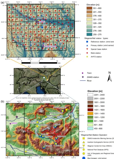
The first study area, the WegenerNet FBR (indicated by the orange-framed white rectangle in the middle panel of Fig. 1, enlarged in a) lies in the Alpine foreland of south-eastern Styria, Austria, centered near the town of Feldbach (46.93◦N, 15.90◦E). It covers a dense grid of 155 meteo-rological stations within an area of about 22 km×16 km, in a hilly terrain, characterized by small differences in altitude (Kirchengast et al., 2014). The typical difference in altitude between the valleys and the crests is about 100 m and the highest peak is the Gleichenberger Kogel, with an elevation of 598 m.
Figure 1.Location of the study areas in Austria (small middle panel betweenaandb), the WegenerNet Feldbach Region (FBR) in the southeast of the state of Styria and the WegenerNet Johnsbachtal (JBT) region in the north of Styria (white rectangles, enlarged inaandb).
(a)The WegenerNet FBR with its 155 meteorological stations, with the legend explaining map characteristics and station types.(b)Map of the WegenerNet JBT region (black rectangle) including its meteorological stations, with the legend explaining map characteristics and station operators.
variability, especially through strong convective activity and severe weather in summer (Kirchengast et al., 2014; Kann et al., 2015a; O et al., 2017, 2018; Schroeer and Kirchen-gast, 2018). The wind fields in this study area are
winds, which lead to cold air pockets, are relevant for this region, which is dominated by agriculture. Especially in fall and winter, the nocturnal cold air production is amplified by temperature inversions in relation to high-pressure weather conditions. In the WegenerNet FBR, hillside locations are thermally preferred to valley locations at night. Results re-lated to the WPG-diagnosed empirical wind fields in the We-generNet FBR can be found in Schlager et al. (2017, 2018).
The second study area, the WegenerNet JBT (indicated by the gray-framed white rectangle in the middle panel of Fig. 1, enlarged in b), is named after the Johnsbachtal river basin (lo-cation of the village of Johnsbach: 47.54◦N, 14.58◦E) and situated in the eastern Alpine region, in the Ennstaler Alps and the Gesäuse National Park, in northern Styria, Austria. The terrain of this mountainous region is characterized by large differences in elevation. The Hochtor, with an eleva-tion of 2369 m, is the highest summit, and the valleys lie roughly at a height of 600 to 800 m (Strasser et al., 2013; Schlager et al., 2018). This region spans an area of about 16 km×17 km and comprises 11 irregularly distributed me-teorological stations including two summit stations at alti-tudes of 2.191 and 1.969 m (Schlager et al., 2018).
The climate is Alpine with mean annual temperatures of around 8 to 0◦C and an annual precipitation of about 1.500 to 1.800 mm from the valley to the summit regions (Wakonigg, 1978; Prettenthaler et al., 2010). Typical for this region are thermally induced local flows and westerly flow synoptic weather conditions. Details related to initial studies and their results as well as to the cooperation and partnerships can be found in Strasser et al. (2013) and in their most up-to-date form in Schlager et al. (2018). Recently, Schlager et al. (2018) computed and evaluated WPG-generated empirical wind fields in this region.
2.2 WegenerNet data
The data acquired from the two WegenerNet regions FBR and JBT are automatically quality controlled and processed by the WegenerNet Processing System (WPS), consisting of four subsystems (Kirchengast et al., 2014): the Com-mand Receive Archiving System transfers raw measurement data via wireless transmission to the WegenerNet database in Graz, the Quality Control System checks the data qual-ity, the Data Product Generator (DPG) generates regular station time series and gridded fields of weather and cli-mate products, and the Visualization and Information Sys-tem offers the data to users via the WegenerNet data portal (https://wegenernet.org/portal/, last access: 2 July 2019).
Besides weather and climate time series, based on a spa-tial interpolation of the station observations, the DPG gener-ates gridded fields of the variables temperature, precipitation, and relative humidity for the WegenerNet FBR. These grid-ded products of the WegenerNet FBR are available to users in near-real time with a latency of about 1–2 h. Kirchengast
et al. (2014) and Kabas (2012) provide detailed information about the subsystems of the WPG.
The DPG furthermore includes a newly developed wind field application, the WPG, as briefly introduced in Sect. 1. The WPG provides high-resolution wind fields for the We-generNet FBR as well as for the WeWe-generNet JBT. The WPG uses the freely available empirical California Meteorological Model (CALMET) as core tool and generates, based on me-teorological observations, terrain elevations, and information about land use and mean wind fields at 10 and 50 m height levels with a spatial resolution of 100 m×100 m and a tem-poral resolution of 30 min, again with a maximum latency of about 1–2 h. In order to keep the meteorological input data of the WPG independent from the data pertaining to the other operational station networks, observations from the Central Institute for Meteorology and Geodynamics (ZAMG) sta-tions (violet stars in Fig. 1a and b) and other external stasta-tions are not used as WPG input. For the WegenerNet FBR, the gridded wind fields are available starting in 2007 and for the WegenerNet JBT starting in 2012. The wind fields at 10 m height level are used for the model intercomparisons.
The CALMET model is a diagnostic model that omits time-consuming integrations of nonlinear equations, such as the governing equations of dynamical models (Truhetz, 2010; Seaman, 2000; Ratto et al., 1994). It is hence not ca-pable of simulating dynamic processes such as flow split-ting and grid-resolved turbulence or of delivering prognos-tic information. Specific parameterizations allow the model to empirically take into account conditions such as the kine-matic effects of terrain, slope flows, and terrain-blocking ef-fects (Scire et al., 1998; Cox et al., 2005; Seaman, 2000). We enhanced the model by implementing methods developed by Bellasio et al. (2005) to as well take into account topo-graphic shading through relief, topotopo-graphic slope and aspect, and the sun position for the estimation of solar radiation. In addition, the modeling of temperature fields is now based on vertical temperature gradients, calculated from meteorologi-cal station observations located at different altitudes, and the influence of vegetation cover is taken into account. Details about these advanced algorithms can be found in Bellasio et al. (2005).
2.3 INCA data
The INCA system has been developed at the ZAMG in Vi-enna, Austria, to provide realistic analyses and nowcasts of quantities of several meteorological variables for the highly mountainous and the overall complex terrain of Austria. In the case of the variable wind, the system operationally gen-erates spatially distributed analysis wind fields in 3-D and for 10 m height above ground with a horizontal grid spacing of 1 km×1 km and a temporal resolution of 1 h.
The basic idea of the INCA wind module is to statisti-cally correct a numerical weather prediction (NWP) model first guess (i.e., in operational mode the latest available NWP model run) with the latest observational data, which do not enter the NWP data assimilation. Thus, the skill of the INCA analysis depends on the station density, their representative-ness, and the spatial distribution of station observations, as well as on the skill of the NWP model providing the first guess. The impact of the NWP model on the analysis skill is further discussed in Kann et al. (2015b).
In this study, NWP model outputs used as a first guess for INCA were generated by the spectral ARPEGE-ALADIN (ALARO) model in a revised version (Wang et al., 2006). ALARO has a horizontal grid spacing of 4.8 km×4.8 km (600×540 grid points) and includes 60 vertical layers up to the 2 hPa level (about 43 km altitude), covering central Eu-rope, eastern France, and the northern part of the Mediter-ranean Sea. It is run with a temporal resolution of 180 s using a hydrostatic semi-implicit semi-Lagrangian dynami-cal solver (Bubnová et al., 1995) and the ALARO-0 physics package, which includes the 3MT microphysics-convection scheme (Gerard and Geleyn, 2005), the Interaction Soil Bio-sphere AtmoBio-sphere (ISBA) force restore 2 L soil scheme (Noilhan and Planton, 1989), and the Actif Calcul de Rayon-nement et Nebulosité (ACRANEB) radiation scheme (Ritter and Geleyn, 1992). Soil temperature and moisture are initial-ized by a 6 h-cycle optimal interpolation data analysis tak-ing into account the latest ALARO forecast as a first guess and 2 m relative humidity and temperature observations from synoptic (SYNOP) and national stations. The 2 m values are transferred to soil variables via empirical relations (Giard and Bazile, 2000). To reduce initial spin-up, a digital filter initial-ization is applied.
The model gets its lateral boundary and atmospheric initial conditions from the high-resolution deterministic operational global integrated forecast system (IFS) of the European Cen-tre for Medium-range Weather Forecasts (ECMWF) model in lagged mode (i.e., ALARO 00:00 UTC is linked to IFS 18:00 UTC of the day before, ALARO 06:00 UTC to IFS 00:00 UTC, etc.). This is due to the rather late availability of the IFS data. Coupling is achieved by one-way nesting via Davies relaxation (Davies, 1976). Sea surface temperature is interpolated from the deterministic IFS model to the ALARO grid. More details about ALARO development and configu-rations can be found in Termonia et al. (2018).
The INCA wind fields have already been evaluated for a moderately hilly region in the north of Austria (47.78– 49◦N, 13.8–17◦E), where the wind analyses show signifi-cantly higher errors compared to the statistical results from other meteorological variables (Haiden et al., 2011). These higher errors mainly root in the limited representativeness of station data, as well as on the low station density, which can be only partly compensated for by INCA’s analysis al-gorithms (Haiden et al., 2011).
In the WegenerNet FBR area, INCA assimilates observa-tions from the ZAMG Feldbach and Bad Gleichenberg sta-tions (violet stars in Fig. 1a) to the NWP’s first guess, and in the WegenerNet JBT region, observations from the ZAMG Admont station are used. However, data from WegenerNet FBR and JBT stations are not used in INCA data assimila-tion and hence the WPG fields can be used for independent evaluation (Haiden et al., 2011).
The coordinate system of the INCA datasets is trans-formed into WGS84/UTM zone 33◦N coordinates. Further-more, we resampled the wind fields at 10 m height levels from the INCA gridding onto the WegenerNet FBR and We-generNet JBT grids, using a bilinear interpolation method. Based on extensive sensitivity tests regarding different inter-polation methods, we concluded that the statistical results do not significantly depend on the interpolation method.
2.4 CCLM data
Regarding the CCLM (Rockel et al., 2008), we use available wind fields generated with the model version 5.0. These wind fields were generated during the course of a previous study and are available for the period 2008 to 2010. The data have a comparatively coarse horizontal resolution of 3 km×3 km on an hourly basis that is nevertheless the highest resolu-tion available to this study. This limited resoluresolu-tion leads to a smoothed orography, which may result in different wind patterns with errors in wind speed or direction. Furthermore, the winds may be displaced by an incorrect position of the topographic slopes (Skok and Hladnik, 2018; Prein et al., 2013b). The CCLM fields are provided for 40 vertical levels. The first level is simulated for 10 m above ground and the last level corresponds to the 100 hPa level (about 16 km alti-tude), whereby the vertical resolution is higher in the bound-ary layer and decreases towards the top level.
and Yamada (Raschendorfer, 2001). Vertical mixing comes from a prognostic formulation of the turbulent kinetic energy (TKE) with a 2.5 closure that accounts for grid- and subgrid-scale water and ice clouds. It uses a statistical cloud scheme for cloud cover and cloud water content (so-called Gaussian closure scheme). Horizontal diffusion follows the Smagorin-sky approach.
Land cover data for CCLM are based on the Global Land Cover 2000 project (EEA, 2016) from SPOT4 satel-lite products (Bartalev et al., 2003). In the model setup used (3 km resolution), deep convection is resolved explic-itly, which means that parameterization for deep convec-tion was switched off. Shallow convecconvec-tion is still parame-terized. In climate research, such simulations are referred to as convection-permitting climate simulations (CPCSs) (Prein et al., 2013a). To minimize decoupling effects from model-internal variability, which usually occurs in large model do-mains and if nudging techniques are not used (Kida et al., 1991), CCLM is operated in a small domain encompassing the greater Alpine region, and it is also driven by ECMWF’s IFS. The data assimilation system IFS includes a wide range of observations and is assumed to provide perfect boundary conditions with a horizontal grid spacing of about 25 km at midlatitudes and at 91 vertical levels (Bechtold et al., 2008). Every 6 h (00:00, 06:00, 12:00, 18:00 UTC) of the IFS data is an analysis field from the assimilation system, and every al-ternate 6 h (03:00, 09:00, 15:00, 21:00 UTC) is a short-range forecast field. This procedure has already been used by Suk-litsch et al. (2011) and keeps the modeled synoptic patterns in agreement with the observed ones.
In the course of the data preparation for the study, CCLM data at 10 m height level were also transformed into WGS84/UTM zone 33N coordinates, resampled and mapped onto the high-resolution WPG grid, and checked for sensitiv-ity with respect to the interpolation method which was also found to be weak (see Sect. 2.3 above).
3 Evaluation events and methods 3.1 Events for wind field evaluation
The WegenerNet, INCA, and CCLM wind fields are inter-compared for two representative types of wind events: ther-mally induced wind events and strong wind events. For this purpose, we defined eight evaluation cases, four for each of the two study areas (Table 1). For the cases shown in Table 1 we use the WegenerNet data as a reference, ex-cept for evaluating the CCLM wind fields for the Wegen-erNet JBT. The reason for this is that the CCLM data used in this study are available from January 2008 to Decem-ber 2009, but the WegenerNet JBT data are available only as of January 2012, since this latter network has been suffi-ciently completed for long-term monitoring only since 2012
(Table 1, cases CCLMvsINCA_therm_JBT and CCLMvs-INCA_strong_JBT).
In both study areas, autochthonous weather conditions mainly lead to thermally induced wind systems, meaning that the wind fields are controlled by small-scale tempera-ture and pressure gradients. These small-scale gradients lead to characteristic interacting systems of air motion, like slope winds and mountain-valley winds, and create complex every-day flow patterns. The autochthonous every-days are characterized by small synoptic influences, cloudless or nearly cloudless skies, low relative humidity and increased radiation fluxes between the Earth surface and the atmosphere (Prettenthaler et al., 2010). Due to frequently occurring temperature inver-sions in relation to clear-sky and high-pressure weather con-ditions in winter, which often lead to a stable atmospheric stratification in the whole WegenerNet FBR and in the valley regions of the WegenerNet JBT, autochthonous days are only selected from spring, summer, and fall (March to October).
The automatic selection of thermally induced and strong wind events is done based on thresholds, which we defined based on sound physical and careful sensitivity checks sum-marized in Table 2. For the estimation of autochthonous days, we compared the observed daytime mean values of wind speed (v) and relative humidity (rh) as well as the nighttime mean values of net radiation (Qn) from selected stations with the respective thresholds. A further criterion for the selec-tion of such days is high daily global radiaselec-tion, which indi-cates fair weather conditions. For this purpose, we compared the daily mean modeled global radiation (Qg,m) for clear-sky conditions with the observed daily mean net radiation (Qn,o) for the WegenerNet FBR and with the observed daily mean global radiation (Qg,o) for the WegenerNet JBT at de-fined station locations (Table 2, reference data). The reason for the comparison ofQg,mwithQn,o for the WegenerNet FBR is that this station network includes no global radiation sensors. Due to the almost linear relationship between the daytimeQg,oandQn,ofor clear-sky conditions, we find that the same selection method can robustly be applied to both study areas by defining different thresholds (Table 2,Qg,m– Qn(g),o). If all criteria are fulfilled for a given day, the data from the entire day are added to the thermally induced wind event dataset, leading to 24 h events (i.e., 24 h mean wind speed values).
The modeling of the global radiation is done based on ESRI’s ArcGIS Area Solar Radiation Tool. This tool is de-signed for local landscape scales and derives the incoming solar radiation based on a digital elevation model. Small dif-ferences of daily mean values betweenQg,mandQn(g),o in-dicate fair weather conditions and high global radiations dur-ing the day. If all criteria are fulfilled for a given day, the data from that day are included in the thermally induced wind events dataset.
com-Table 1.Characteristics of wind field evaluation cases used for the WegenerNet, INCA, and CCLM intercomparisons (top half for the WegenerNet FBR; bottom half for the WegenerNet JBT region).
Evaluation Modeled Reference
case Type Region dataset dataset Period WegenerNet FBR
INCAvsWN_therm_FBR thermally FBR INCA WN 2008–2017 INCAvsWN_strong_FBR strong FBR INCA WN 2008–2017 CCLMvsWN_therm_FBR thermally FBR CCLM WN 2008–2010 CCLMvsWN_strong_FBR strong FBR CCLM WN 2008–2010
WegenerNet JBT
INCAvsWN_therm_JBT thermally JBT INCA WN 2012–2017 INCAvsWN_strong_JBT strong JBT INCA WN 2012–2017 CCLMvsINCA_therm_JBT thermally JBT CCLM INCA 2008–2010 CCLMvsINCA_strong_JBT strong JBT CCLM INCA 2008–2010
Table 2.Limits for the selection of thermally induced or strong wind events for the defined evaluation cases shown in Table 1 (top half for the WegenerNet FBR; bottom half for the WegenerNet JBT).
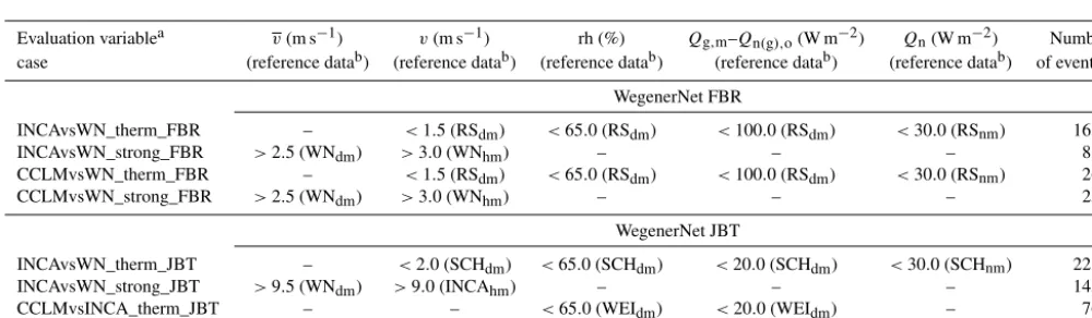
Evaluation variablea v(m s−1) v(m s−1) rh (%) Qg,m–Qn(g),o(W m−2) Qn(W m−2) Number
case (reference datab) (reference datab) (reference datab) (reference datab) (reference datab) of eventsc WegenerNet FBR
INCAvsWN_therm_FBR – <1.5 (RSdm) <65.0 (RSdm) <100.0 (RSdm) <30.0 (RSnm) 1632
INCAvsWN_strong_FBR >2.5 (WNdm) >3.0 (WNhm) – – – 830
CCLMvsWN_therm_FBR – <1.5 (RSdm) <65.0 (RSdm) <100.0 (RSdm) <30.0 (RSnm) 264
CCLMvsWN_strong_FBR >2.5 (WNdm) >3.0 (WNhm) – – – 259
WegenerNet JBT
INCAvsWN_therm_JBT – <2.0 (SCHdm) <65.0 (SCHdm) <20.0 (SCHdm) <30.0 (SCHnm) 2232
INCAvsWN_strong_JBT >9.5 (WNdm) >9.0 (INCAhm) – – – 1450
CCLMvsINCA_therm_JBT – – <65.0 (WEIdm) <20.0 (WEIdm) – 768
CCLMvsINCA_strong_JBT >6.0 (INCAdm) >6.0 (INCAhm) – – – 182
av: average wind speed;v: wind speed; rh: relative humidity;Qg,m–Q
(n)g,o: difference between mean modeled global radiation (Qg,m) and observed net radiation (Qn,o) for the WegenerNet FBR and difference betweenQg,mand observed global radiation (Qg,o) for the WegenerNet JBT;Qn: net radiation.bRS: Reference Station (Nr. 77); SCH: Schroeckalm station; WEI: Weidendom
station; dm: daytime mean value from observations (from sunrise until sunset); nm: nighttime mean value from observations (from sunset until sunrise); WNdm: daily mean value from gridded
WegenerNet wind speed; WNhm: hourly mean value from gridded WegenerNet wind speed; INCAdm: daily mean value from gridded INCA wind speed; INCAhm: hourly mean value from gridded
INCA wind speed.cHourly wind events; i.e., hours are used as the base period for the statistical analysis.
paring hourly mean values from gridded reference datasets with defined minimum wind speeds. These preselected days were estimated by comparing the daily average wind speed from the gridded datasets with a defined minimum average wind speed (Table 2,vandvfor strong wind speed cases). If the hourly mean value of this reference dataset is larger than the defined minimum wind speed, the data of this reference dataset and the corresponding model dataset are used as part of the hourly event data for evaluating strong wind events. 3.2 Statistical evaluation methods
In order to account for spatial differences and displacements between the model and the reference data and to analyze wind speed and direction in a combined way, we apply a novel wind verification methodology. This methodology ex-tends the fractions skill score (FSS), a spatial verification metric developed by Roberts (2008), which is classified as
a neighborhood-based approach and originally used for veri-fying precipitation. The FSS is based on the assumption that a model is useful when the model data and the corresponding reference data show a similar spatial frequency of precipita-tion events, which alleviates the requirement of the models to predict the events at exactly correct positions, which is an unduly strict assumption. Furthermore, this metric avoids the double-penalty problem and provides scale-dependent infor-mation about the level of model skill (Gilleland et al., 2010; Roberts, 2008).
successively at each grid point, whereby the area outside the domain is assumed to contain no wind class. In terms of the FSS value, it is a 0-to-1 normalized metric; i.e., the lower limit of the FSS is 0 and the upper limit +1, with values approaching+1 representing a better degree of model per-formance.
The extended version of the FSS is called the wind frac-tions skill score, denoted WFSS, which has been developed by Skok and Hladnik (2018). The score is calculated based on user-defined wind classes. The definition of these classes is partly subjective and can significantly affect the WFSS. The wind vector field should be classified in such a way, that the definition reflects what a user wants to analyze. For ex-ample, a complex terrain leads to strong changes in wind di-rections; therefore, it is reasonable to define smaller class in-tervals regarding the wind directions. For upper-level winds the focus could be more on the magnitude of wind speed.
We defined eight wind direction classes with an interval size of 45◦ for a range of three wind speed categories, as shown in the wind roses of Fig. 2. Wind speeds<0.5 m s−1 were classified as calm, independently of the wind direc-tion. The small interval size of 45◦was chosen to be able to capture the varying wind directions in the study areas, espe-cially for thermally induced winds. Because of the generally much lower wind speeds in WegenerNet FBR, we defined a smaller interval size of the wind speed categories for this re-gion (Fig. 2a and b, lower panels) than for the WegenerNet JBT (Fig. 2c and d, lower panels).
Table 3 includes the equations for the calculation of the WFSS and the asymptotic WFSS (AWFSS). This AWFSS will always be reached for a neighborhood size ≥2N−1, whereNis the number of grid points of the largest domain size. At such a large neighborhood size, the estimated frac-tions within the domain are the same at all locafrac-tions, and further enlarging this size will not affect the WFSS. A bias always leads to an AWFSS value <1, which indicates sys-tematic differences in the frequency of wind classes between the model and the reference wind classification.
The WFSS is calculated for each hourly field for the se-lected events. The event-averaged score values are calculated based on averaging these 1 h event WFSS values over all the hourly events within the analyzed multiyear period, for each evaluation case listed in Table 1.
As briefly explained above, the chosen thresholds of the classification and the number of classes influence the score. We found, in particular, that the wind direction thresholds can have a strong impact on the score values. For example, a small change in the wind direction value from prevailing northwesterly winds, which are close to a threshold to dis-tinguish between W and N, could dramatically change the WFSS value. Such a small error in the model data could in-dicate a poor modeling performance, whereas a human ana-lyst would assess the forecast as reasonably good. To avoid this problem we calculated the hourly WFSS for every ro-tation between 0 and 45◦ with an interval size of 5◦ (nine
trail classes), in addition to the original class definition. As a next step, the maximum values of the hourly score values at each neighborhood size are always used for computing the final case-averaged score values. We applied this approach for 7597 selected events in total (Table 2, number of events) and estimated the case-averaged score value for each of the eight evaluation cases. A more detailed description of the wind fractions skill score metric can be found in Skok and Hladnik (2018).
Furthermore, we applied traditional grid-point-based sta-tistical performance measures such as bias, root-mean-square error, and others, to each evaluation case. All statistical per-formance metrics used in this study are summarized in Ta-ble 3.
4 Results
4.1 Evaluation for selected wind events
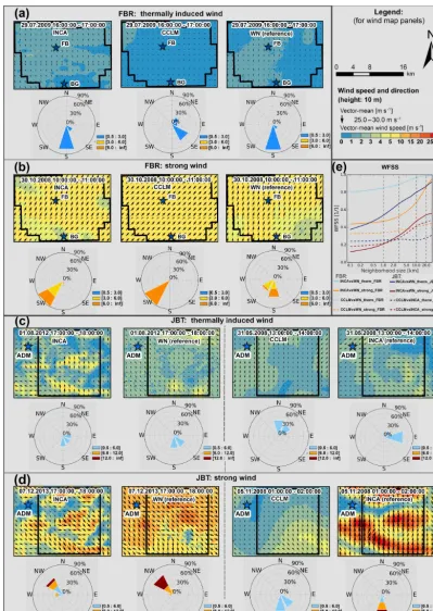
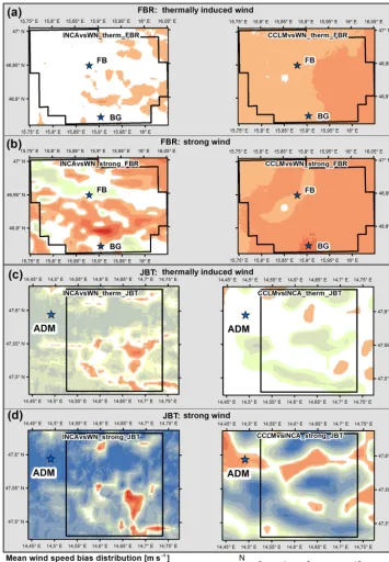
Figure 2a–d illustrate typical examples of modeled wind fields (upper rows of panels) and the corresponding wind roses of relative frequency of wind directions divided by wind speed categories (lower rows of panels) from selected representative evaluation events. Each panel depicts the mod-eled and the associated reference data for the WegenerNet FBR (Fig. 2a and b) and the WegenerNet JBT (Fig. 2c and d), for thermally induced (Fig. 2a and c) and strong wind events (Fig. 2b and d). Figure 2e shows the WFSS values of these examples, estimated as explained in Sect. 3.2 above.
The thermally induced wind event on the 29 July 2009 from 16:00 to 17:00 UTC for the WegenerNet FBR (Fig. 2a) shows thermally driven regional flows caused by Alpine pumping. This flow is called “Antirandgebirgswind”, which arises usually in the afternoon as southerly wind with max-imum wind speeds of about 2.5 m s−1. The Antirandge-birgswind is a compensating flow between the bordering mountains of the eastern Alps, and the hilly countryside re-gion of southeastern Styria (called Riedelland), which com-prises the WegenerNet FBR (Wakonigg, 1978). The INCA (upper-left panel of Fig. 2a) and the WegenerNet wind fields (upper-right panel of Fig. 2a) show a similar distribution with generally low wind speeds and prevailing southerly wind di-rections. The intercomparison of these INCA data with We-generNet data for this event shows the largest WFSS val-ues for all neighborhood sizes, which indicates a good over-lap of the wind classes (Fig. 2e, INCAvsWN_therm_FBR). Furthermore, it shows a nearly perfect asymptotic value of about 0.99. This large AWFSS indicates a very small bias, which is also reflected by the similar wind classification re-sults (lower-left and lower-right panel of Fig. 2a).
Table 3.Statistical performance parameters used for the intercomparison of the wind field modeling results.
Parameter Equation Remarks
Wind fractions skill score WFSS=1− P
k P
i,j[Ok(i,j )−Mk(i,j )]2 P
k n
P
i,jOk(i,j )2+Pi,jMk(i,j )2
o Ok: fraction values for observations for wind classkat locationi,j;Mk: fraction values for model data for wind classkat locationi,
j(Skok and Hladnik, 2018; Roberts, 2008)
Asymptotic WFSS AWFSS=1−
P kfkO−fkM
2 P k n fO k 2+fM
k
2o f
O
k : frequency of wind classkin the obser-vations;fkM: frequency of wind classkin the model data (Skok and Hladnik, 2018)
Bias B= 1
N PN
i=1 vm,i−vo,i
vm: modeled wind speed;vo: observed wind
speed
Standard deviation of observed wind speed SDo=
q
1
(N−1) PN
i=1(vo,i−vo)2 vo: observed wind speed;vo: mean observed
wind speed
Root-mean-square error RMSE=
q
1
N PN
i=1(vm,i−vo,i)2 vm: modeled wind speed;vo: observed wind
speed
Correlation coefficient R= 1
(N−1) PN
i=1
v
m,i−vm
σm
vo,i−vo
σo
vm: modeled wind speed;vm: mean modeled
wind speed; vo: observed wind speed;vo:
mean observed wind speed;σm: standard
de-viation of modeled wind speed;σo: standard
deviation of observed wind speed Mean absolute error of wind direction MAEdir=N1
PN i=1
arccos[cos(φm,i−φo,i)] φm: modeled wind direction;φo: observed
wind direction
generNet data can be observed (middle and lower-right panel of Fig. 2a). This shift is reflected by small WFSS values at all neighborhood sizes, especially below a scale of 10 km. The AWFSS shows the largest value of all CCLM intercomparisons but is still low compared to INCA evaluation cases, which indicates a large bias (Fig. 2e, CCLMvsWN_therm_FBR). Evidently, this regional climate wind field modeling at 3 km grid spacing is not adequately representative for the given challenging hilly terrain.
The strong wind speed event in the WegenerNet FBR on the 30 October 2008 from 10:00 to 11:00 UTC led to south-westerly to southerly winds (Fig. 2b). The INCA model data and the WegenerNet reference data show maximum 1 h vector-mean wind speeds of around 9–10 m s−1 (upper-left and right panel of Fig. 2b). Regarding the wind direc-tions, differences in the wind sectors can be observed (lower-left and right panel of Fig. 2b). The INCA data show wind directions mainly from the SW sector (lower-left panel), while the WegenerNet data show wind directions from the S and SW sectors (lower-right panel). The WFSS for this case shows small values at small neighborhood sizes and increases with increasing neighborhood size (Fig. 2e, IN-CAvsWN_strong_FBR). These low WFSS values are mainly caused by the differences in wind direction classes, espe-cially in the southern part of the domain and through some spatial displacements in wind speed classes. Despite low WFSS values at small neighborhood sizes caused by differ-ences in wind sectors, the AWFSS shows a high asymptotic
value (AWFSS>0.97). This high value is caused by the pre-vailing wind directions in the WegenerNet data, which are close to the threshold values for distinguishing between S and the SW. Hence, in this case, the 5◦azimuthal class rota-tion procedure avoids lower score values.
Regarding the CCLM data (lower-middle panel of Fig. 2b), the whole wind field shows wind speeds from about 6.5 to 7.5 m s−1and is therefore assigned to the wind class with wind speeds higher than 6 m s−1, whereas, for the WegenerNet wind fields, a large proportion is assigned to the class with wind speeds from 3 to 6 m s−1 of this re-gion (Fig. 2e, CCLMvsWN_strong_FBR) and indicates that the dynamically modeled CCLM wind speeds are system-atically overestimated relative to the empirically diagnosed wind speeds.
This discrepancy leads to the smallest WFSS val-ues at all neighborhood sizes for this region (Fig. 2e, CCLMvsWN_strong_FBR) and indicates that the dynami-cally modeled CCLM wind speeds are systematidynami-cally under-estimated relative to the empirically diagnosed wind speeds for this hourly event.
in-dicates overlapping areas at this neighborhood size, equal to the horizontal resolution of the INCA analysis (Fig. 2e, IN-CAvsWN_therm_JBT). The large AWFSS value again indi-cates a small bias, which is also reflected by the similar wind classification shown in the wind roses of the correspond-ing lower-left panels of Fig. 2c. The high asymptotic value (AWFSS>0.9) indicates a small bias and that the WFSS is mostly influenced by the spatial displacement.
In a further example of a thermally induced wind event on the 31 May 2008, we intercompare the CCLM with INCA wind fields (right panels of Fig. 2c). Especially in the CCLM, the smoothed terrain leads to uniform wind speeds and direc-tions. Regarding the INCA wind fields, some variability in wind speed can be observed, with higher values in the sum-mit regions and lower values at lower altitudes in the val-leys of this region. Furthermore, a valley wind in the Enns valley is simulated by INCA. Probably the analysis part of the INCA model with its higher-resolved digital elevation model (DEM) and assimilated ZAMG observations leads to a somewhat better representation of the wind field. Comparing wind directions, the largest part of the CCLM modeled flow is from the N and NE sectors, while the INCA system esti-mated wind directions mainly from the E sector and partly from the NE and SE sectors (bottom right panels of Fig. 2c). This simplistic pattern of wind directions in CCLM leads to low WFSS values for all neighborhood sizes, including the lowest asymptotic value of all examples, indicating a very poor representation of the wind field by the dynamical mod-eling of the CCLM in this challenging mountainous terrain.
The strong wind speed event for the WegenerNet JBT on the 7 December 2013 is caused by northwesterly weather conditions. These synoptic-scale flow conditions led to strong wind speeds with maximum 1 h mean wind speeds of around 20 m s−1from 17:00 to 18:00 UTC. Both the INCA and the WegenerNet wind fields show wind directions mainly from the NW, with some proportions from the N and the W sectors, caused by a channeling of the air flow through the pronounced valleys of this study area. The INCA wind fields show much lower wind speeds in the valley regions com-pared to the WegenerNet wind fields, resulting from the ob-servations of the ZAMG Admont (ADM) station that flow into the INCA analysis but are considered far off the area and not used by the diagnostic modeling (upper-left panels of Fig. 2d). As the neighborhood size increases, the WFSS also increases, but due to spatial displacements, the values are generally low (Fig. 2e, INCAvsWN_strong_JBT). The low AWFSS value is caused by the differences in wind speed categories (lower-left panels of Fig. 2d).
For the 5 November 2008 we intercompare the CCLM wind fields with INCA wind fields from 01:00 to 02:00 UTC, for a strong wind speed event (right panels of Fig. 2d). In this example, the influence of the smoothed terrain caused by the coarse horizontal resolution of the CCLM becomes obvious. This smoothed topography results in systemat-ically lower wind speeds compared to the INCA wind
fields. The WFSS shows similar results to the previous IN-CAvsWN_strong_JBT evaluation, with small values at all neighborhood sizes (Fig. 2e, CCLMvsINCA_strong_JBT), indicating the clear limits of the CCLM dynamical model-ing fields also for strong wind events.
4.2 Statistical evaluation results
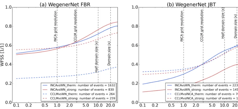
The statistical event-averaged WFSS values from the large ensemble of events over multiple years are represented for each evaluation case in Fig. 3. Overall, the WFSS values show a monotonic increase with neighborhood size for all cases so that the AWFSS is the largest value, indicating rela-tively the best performance at large scales.
For the WegenerNet FBR, the statistical WFSS values, cal-culated for the INCA wind fields compared to the Wegen-erNet wind fields, shows nearly the same behavior for both the thermally induced and strong wind events (Fig. 3a, IN-CAvsWN_therm_FBR and INCAvsWN_strong_FBR). The WFSS values for these cases indicate a reasonably good spa-tial matching at all neighborhood sizes. Furthermore, the AWFSS values are higher than 0.8, reflecting generally small INCA biases of wind classes.
The statistical WFSS estimated for the CCLMvsWN_therm_FBR case indicates that the CCLM clearly and systematically underperforms in the case of thermally induced wind events for the WegenerNet FBR. Evidently, due to the coarse horizontal resolution of the wind fields, the CCLM wind fields appear fundamentally unable to capture the varying wind directions for such events in this region. For the CCLMvsWN_strong_FBR case, however the results indicate a similar spatial matching as for the INCAvsWN_therm_FBR and INCAvsWN_strong_FBR cases, just with a somewhat higher bias of wind class differences. This similar performance despite the coarser horizontal resolution of the CCLM model is explained through a weaker influence of the terrain on the wind fields under strong wind conditions in this region.
Because of the challenging terrain of the WegenerNet JBT, the statistical WFSS values are generally low for this re-gion, signalling large biases (Fig. 3b). These biases are in-dicated by low asymptotic values, which tend to be between 0.61 and 0.64, except for the INCAvsWN_strong_JBT case, which shows an even lower value (AWFSS=0.39).
The spatial displacement and the biases for the IN-CAvsWN_therm_JBT case are mainly caused by the differ-ences in wind directions for these thermally induced wind events. Especially at small neighborhood sizes at the 1 km scale, WFSS values indicate large spatial displacements.
overesti-Figure 3.The event-averaged wind fractions skill score (WFSS) results for the WegenerNet FBR(a), compared to the WegenerNet JBT
(b), for the four defined evaluation cases in each region (see legend; indicating also the number of events included). See Table 1 for more information on the evaluation cases.
mated WegenerNet wind speeds in the Enns valley somewhat reinforces the difference between the INCA and the Wegen-erNet wind speeds. These differences in wind speed espe-cially in the valley and the summit regions become obvious in Fig. 4c and d and are discussed in further detail below.
The intercomparison of the CCLM wind fields with INCA delivers nearly the same (low) WFSS values for both types of wind events. In the case of thermally induced events (CCLMvsINCA_therm_JBT), the spatial displacements and biases are mainly caused due to differences in wind direc-tions. For strong wind events (CCLMvsINCA_strong_JBT), the smoothed terrain caused by the coarse resolution of the CCLM leads to systematically underestimated wind speeds.
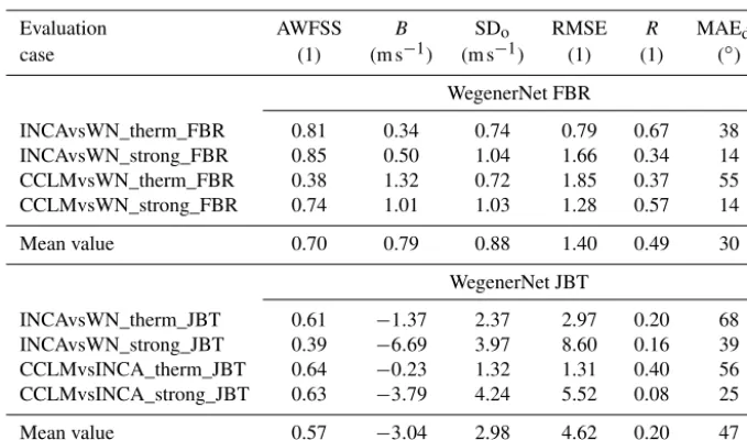
Table 4 summarizes, in addition to the AWFSS values, the results estimated with traditional statistical methods of the INCA analysis and CCLM dynamical fields. Due to the less challenging region of the WegenerNet FBR, all tra-ditional statistical parameters show better performance for this region compared to the WegenerNet JBT. The absolute-value statistical metrics (biasB, standard deviation SDo, root-mean-square error RMSE) applied to the hourly vector-mean wind speeds show higher values for the WegenerNet JBT, resulting from the generally higher wind speeds in addition to the effects of the complex mountainous terrain on the wind fields in this region. The B values are slightly posi-tive for the WegenerNet FBR and negaposi-tive for the Wegen-erNet JBT. The substantially negative B value for the IN-CAvsWN_strong_JBT case again reflects the underestima-tion of wind speed in the valleys, as explained above. Further-more, the CCLMvsINCA_strong_JBT intercomparison also shows a negative bias, caused by the coarse resolution of the
CCLM, which leads to lower wind speeds for strong wind events.
The RMSE values range from 0.79 to 1.85 m s−1for the WegenerNet FBR and from 1.3 to 8.6 m s−1 for the We-generNet JBT. The high value of 8.6 m s−1 for the IN-CAvsWN_strong_JBT case is caused by the underestimation of wind speed in the valleys as well as the overestimation in the summit regions by the INCA model. The meanRvalues show a better correlation for the WegenerNet FBR than for the WegenerNet JBT. The mean absolute error of wind direc-tion (MAEdir) applied to hourly vector-mean wind directions also shows better performance (INCA and CCLM fields) for the WegenerNet FBR. Due to the varying wind direc-tions caused by thermally induced circuladirec-tions, the MAEdiris higher for such events for both study areas, with the highest value of 68◦for the INCAvsWN_therm_JBT case.
Figure 4 shows the mean wind speed bias spatial distri-butions for all evaluation cases, for the WegenerNet FBR (Fig. 4a and b) and the WegenerNet JBT (Fig. 4c and d). The distribution for the INCAvsWN_therm_FBR case, the case for thermally induced wind events for the WegenerNet FBR, shows large areas with nearly noBvalues (left panel of Fig. 4a). The maximumBvalue for this case can be observed in the area of the Gleichenberger Kogel, north of the ZAMG Bad Gleichenberg station with a value of around 1.4 m s−1. The evaluation of the CCLM for the same thermally induced events shows an overestimation of wind speeds for the whole study area, withBvalues from 0.5 to 1 m s−1in the western part and from 1 to about 1.4 m s−1in the eastern part of the study area (right panel of Fig. 4a).
Figure 4.Mean wind speed bias distribution for the WegenertNet FBR(a, b)and the WegenerNet JBT(c, d):(a, b)INCA versus WegnerNet (left) and CCLM versus WegenerNet (right) for(a)thermally induced wind events and(b)strong wind events and(c, d)WegenerNet versus INCA (left) and CCLM versus INCA (right) for(c)thermally induced wind events and(d)strong wind events.
simulated for this region, which lead to a more dominant oro-graphic speedup effect. Due to orooro-graphic smoothing, flow-over patterns are generally more frequent than flow-around patterns, especially for the WegenerNet FBR with its small differences in altitude (Taylor et al., 1987).
Table 4.Statistical performance measures calculated for the evaluation cases from Table 1, for the WegenerNet FBR and the WegenerNet JBT region. See Table 3 for more information on the calculation of the parameters.
Evaluation AWFSS B SDo RMSE R MAEdir
case (1) (m s−1) (m s−1) (1) (1) (◦) WegenerNet FBR
INCAvsWN_therm_FBR 0.81 0.34 0.74 0.79 0.67 38 INCAvsWN_strong_FBR 0.85 0.50 1.04 1.66 0.34 14 CCLMvsWN_therm_FBR 0.38 1.32 0.72 1.85 0.37 55 CCLMvsWN_strong_FBR 0.74 1.01 1.03 1.28 0.57 14 Mean value 0.70 0.79 0.88 1.40 0.49 30
WegenerNet JBT
INCAvsWN_therm_JBT 0.61 −1.37 2.37 2.97 0.20 68 INCAvsWN_strong_JBT 0.39 −6.69 3.97 8.60 0.16 39 CCLMvsINCA_therm_JBT 0.64 −0.23 1.32 1.31 0.40 56 CCLMvsINCA_strong_JBT 0.63 −3.79 4.24 5.52 0.08 25 Mean value 0.57 −3.04 2.98 4.62 0.20 47
Gleichenberger Kogel. Overall positiveB values of CCLM dynamical wind speed fields for strong wind events are seen in the right panel of Fig. 4b, showing the systematic overes-timating by CCLM fields in this case. These largeB values are probably also due to the speedup effect explained for the above case CCLMvsWN_therm_FBR.
For the WegenerNet JBT, the strong influence of the terrain on the INCA-analyzed wind speeds can be observed in all evaluation cases in this region. The evaluation of the INCA model for thermally induced wind events exhibits negative B values in the valleys, whereby positive values partly oc-cur in the summit regions (left panel of Fig. 4c). At lower elevations, the intercomparison of the CCLM with the INCA model shows nearly noBvalues for thermally induced events (right panel of Fig. 4c). Furthermore, small negativeBvalues in the summit regions and some spots with positive values can be observed for this case. Due to these small bias values, similar results to these ones can be expected for a comparison of CCLM with WegenerNet data.
Similar bias distribution patterns as for the INCA evalua-tion for thermally induced wind events are present for strong wind events in the INCAvsWN_strong_JBT case, but this time with strong negative and positiveBvalues ranging from
−14.4 to 4.9 m s−1(left panel of Fig. 4d). These strong neg-ative B values are again caused by the severely underesti-mated INCA wind speeds and the somewhat overestiunderesti-mated WegenerNet wind speeds in the valley regions of the Wegen-erNet JBT.
Opposite patterns can be seen for the intercomparison of the CCLM with the INCA model. This intercomparison ex-hibits small positive values in the valley regions and strong negative values in the summit regions (right panel of Fig. 4d). The main reason for these strong negative B values is the
coarse resolution of the CCLM data and the resulting un-derestimation of wind speeds for strong wind events, as ex-plained above. The negativeB values are likely caused by negative orographic speedup effects, which are preferred in flow-around patterns and flow-splitting patterns that occur especially when the differences in the altitude of ridges of mountains are large (Hewer, 1998).
5 Conclusions
In this work we evaluated wind fields generated by two different modeling systems against empirically diagnosed wind fields from WegenerNet high-density network data: the INCA analysis system of the Austrian weather service Cen-tral Institute for Meteorology and Geodynamics (ZAMG) (Haiden et al., 2011) and the non-hydrostatic Consortium for Small Scale Modeling Model in Climate Mode (CCLM) (Schättler et al., 2016). The INCA wind fields have a hori-zontal resolution of 1 km×1 km, and in the case of CCLM, 3 km×3 km horizontal resolution was available. In both cases, the temporal resolution is 1 h. The empirical high-resolution wind fields from the WegenerNet were generated by the WegenerNet Wind Product Generator (WPG), recently developed by Schlager et al. (2017, 2018).
The evaluation of the INCA and the CCLM wind fields was based on classifying the data separately into thermally induced and strong wind events. In the case of the INCA evaluation, we could select wind events within the period 2008–2017 for the WegenerNet FBR and within 2012–2017 for the WegenerNet JBT. For evaluating the CCLM data, events from the period 2008–2010 were selected for both study areas. Due to WegenerNet JBT wind fields not yet being available within 2008–2010, we intercompared the CCLM wind fields with INCA wind fields in this region.
Besides traditional performance measures such as bias, root-mean-square error, correlation coefficient, and mean ab-solute error of wind direction, in particular we applied a spatial wind verification methodology called the wind frac-tions skill score (WFSS) (Skok and Hladnik, 2018). This new score was used to detect spatial displacements of wind pat-terns and biases based on predefined wind speed and direc-tion classes. The WFSS avoids the double-penalty problem and is able to distinguish between a “near miss” and large displacements between modeled and reference wind fields. Furthermore, a spatial-scale-dependent skill is determined by this score.
Due to the less challenging terrain of the Alpine fore-land region, all statistical performance measures showed bet-ter INCA and CCLM performance for the WegenerNet FBR than for the challenging mountainous region of WegenerNet JBT. The spatial verification of all evaluation cases indicates an increasing skill with increasing scale (neighborhood size). For both study areas, the traditional statistical performance measures, applied to the wind speed, mostly show better per-formance of INCA and CCLM for thermally induced wind events than for strong wind events. On the other hand, the re-sults related to wind direction indicate a better performance for strong wind events than for thermally induced events.
More specifically, the verification for the WegenerNet FBR shows that the INCA analysis wind fields are more skill-ful than the CCLM dynamical wind fields in this region. The INCA verification indicates a reasonably good performance for both thermally induced and strong wind events.
The CCLM clearly performs less well in the case of ther-mally induced wind events for this region. The reason for this weak performance is the limited resolution of the wind field dataset from this model. Although the difference in the numerical resolution between INCA (1 km grid spacing) and CCLM (3 km grid spacing) is only a factor of 3, CCLM is not able to resolve small-scale wind patterns. This occurs for multiple reasons: (1) due to the third-order advection scheme with its horizontal diffusion damping, the effective resolution in CCLM is several times coarser than the numeric grid spac-ing (Ogaja and Will, 2016); (2) the orography is smoothed as well, so that individual mountain ridge and valley structures are removed. For example, the mountain peak of the Hochtor with its 2396 m elevation at the center of the WegenerNet JBT region is lowered by about 500 m in the CCLM model.
Hence, with the resolution of 3 km×3 km, the fields are not able to resolve the varying wind speeds and directions caused by thermally driven circulations. The wind speeds are overestimated by this model for both thermally induced and strong wind events, and large differences in wind directions are found for thermally induced events.
For the WegenerNet JBT region, the verification shows generally large spatial displacements at all scales and strong biases in wind classes for all evaluation cases. In the case of the INCA evaluation, large wind direction deviations for thermally induced wind events indicate that the analysis fields are not able to adequately capture the varying wind pat-terns such as slope and valley winds, which are rooted in the sparse station density to which INCA can be anchored and the coarse horizontal resolution of the first guess provided by the ARPEGE-ALADIN (ALARO) model in this complex-terrain region. Furthermore, the statistics show an substantial underestimation of wind speeds in the valleys and overesti-mated wind speeds in parts of the summit regions for both types of wind events.
The intercomparison of the CCLM dynamical fields with the INCA analysis fields for thermally induced wind events reflects the disadvantage of smoothed terrain, which is caused by the limited effective resolution being several times coarser than the 3 km×3 km grid spacing of the CCLM as already noted above. Improvements can be expected from the latest developments in the numerical core of CCLM by Ogaja and Will (2016), which have enabled an improvement of the effective resolution by a factor of 2 by introducing a fourth-order advection scheme that allows us to circumvent the horizontal diffusion damping.
Based on these findings and underpinning the results of Haiden et al. (2011), we suggest that additional observed wind information in the summit and valley regions, espe-cially in a complex terrain like the WegenerNet JBT, and a more comprehensive use of wind-constraining satellite data as well as a higher-resolution regional climate model (RCM) could help to systematically improve the INCA-analyzed wind fields. At higher resolutions, the topographic shading through the terrain becomes increasingly impor-tant, especially for the simulation of thermally induced wind events. Such methods have not yet been implemented into the ALARO model but may help to generate more realistic wind fields in the future.
Related to the CCLM dynamical modeling, a verification of CCLM-generated higher-resolution 1 km×1 km wind fields and the application of the new fourth-order advec-tion scheme from Ogaja and Will (2016) in a convecadvec-tion- convection-permitting configuration would also be a promising issue for further investigations of how this may improve the modeling of wind patterns in a complex terrain.
over-estimation of WegenerNet wind speeds in the Enns valley, especially for strong wind events. In the WegenerNet FBR just recently (in May 2018), another wind station was added in the Raab valley (station Nr. 155 1b), which will further improve the WPG-derived fields in future. This adds further value to a valuable reference for the evaluation of important other data products such as the INCA operational analysis and dynamical climate model fields.
Code availability. The CALMET 6.5.0 model code is available from the website http://www.src.com (last access: 2 July 2019; Exponent, Inc., 2018). The INCA and the WPG code are not in the public domain and cannot be distributed. The source code for the CCLM is available on request via the website https: //www.clm-community.eu (last access: 2 July 2019; Deutscher Wetterdienst, 2019). The code for the calculation of the wind FSS is available as part of the SpatialVx package (function cal-culate_FSSwind). SpatialVx is a R software package made by Eric Gilleland that enables the calculation of a large number of spatial verification scores (https://cran.r-project.org/package= SpatialVx, last access: 2 July 2019; Gilleland, 2019).
Data availability. CORINE land cover data for the study area were taken from https://www.eea.europa.eu/ (last access: 2 July 2019; EEA, 2016), digital elevation model data from http://www. landesentwicklung.steiermark.at/cms/ziel/141976122/DE/ (last ac-cess: 2 July 2019; Land Steiermark, 2019), and WegenerNet data from https://wegenernet.org/portal/ (last access: 2 July 2019; We-gener Center, 2019). The WeWe-generNet data contain the WPG wind field output data as introduced in this study. The INCA data are available on request from the Central Institute for Meteorol-ogy and Geodynamics ([email protected]). CCLM data are avail-able on request from the Wegener Center, University of Graz ([email protected]).
Author contributions. CS collected the data, performed the analy-ses and modeling, created the figures, and wrote the first draft of the paper. GK provided guidance and advice on all aspects of the study and significantly contributed to the text. JF provided guidance on technical aspects of the WegenerNet networks and its data charac-teristics and contributed to the text. AK provided INCA-related ad-vice and contributed to the INCA part of the text, and HT provided information and advice on the CCLM setup and characteristics and contributed in particular to the CCLM part of the text. All authors commented on the final version of the paper.
Competing interests. The authors declare that they have no conflict of interest.
Acknowledgements. The authors thank Gregor Skok (Depart-ment of Physics, University of Ljubljana), for providing the R code to calculate the wind fractions skill score. Furthermore, the authors acknowledge the data providers at the Central Institute for
Mete-orology and Geodynamics (ZAMG) for the Integrated Nowcast-ing through Comprehensive Analysis (INCA) dataset. Andras Csaki (Wegener Center, University of Graz) is thanked for performing the CCLM modeling and extracting the wind field data. The authors are also grateful to the Jülich Supercomputing Centre (JSC) and the Vienna Scientific Cluster (VSC) for providing the necessary HPC resources. WegenerNet funding is provided by the Austrian Min-istry for Science and Research, the University of Graz, the state of Styria (which also included European Union regional development funds), and the city of Graz; detailed information can be found on-line (http://www.wegcenter.at/wegenernet, last access: 2 July 2019). The CCLM simulation was funded by the Austrian Science Fund (FWF) under project NHCM-2 (project number P24758-N29).
Review statement. This paper was edited by Richard Neale and re-viewed by two anonymous referees.
References
Abdel-Aal, R., Elhadidy, M., and Shaahid, S.: Modeling and forecasting the mean hourly wind speed time series using GMDH-based abductive networks, Renew. Ener., 34, 1686– 1699, https://doi.org/10.1016/j.renene.2009.01.001, 2009. Awan, N. K., Truhetz, H., and Gobiet, A.: Parameterization-induced
error characteristics of MM5 and WRF operated in climate mode over the alpine region: An ensemble-based analysis, J. Climate, 24, 3107–3123, https://doi.org/10.1175/2011JCLI3674.1, 2011. Bartalev, S., Belward, A., Ershov, D., and S. Isaev, A.:
A new SPOT4-VEGETATION derived land cover map of Northern Eurasia, Int. J. Remote Sens., 24, 1977–1982, https://doi.org/10.1080/0143116031000066297, 2003.
Bechtold, P., Köhler, M., Jung, T., Doblas-Reyes, F., Leutbecher, M., Rodwell, M. J., Vitart, F., and Balsamo, G.: Advances in sim-ulating atmospheric variability with the ECMWF model: From synoptic to decadal time-scales, Q. J. Roy. Meteor. Soc., 134, 1337–1351, https://doi.org/10.1002/qj.289, 2008.
Bellasio, R., Maffeis, G., Scire, J. S., Longoni, M. G., Bianconi, R., and Quaranta, N.: Algorithms to Account for Topographic Shad-ing Effects and Surface Temperature Dependence on Terrain El-evation in Diagnostic Meteorological Models, Bound.-Lay. Me-teor., 114, 595–614, https://doi.org/10.1007/s10546-004-1670-6, 2005.
Böhm, U., Kücken, M., Ahrens, W., Block, A., Hauffe, D., Keuler, B., Rockel, B., and Will, A.: CLM-The Climate Ver-sion of LM: Brief Description and Long-Term Applications, 225–236, Deutscher Wetterdienst (DWD), 6 Edn., available at: http://www.cosmo-model.org/content/model/documentation/ newsLetters/newsLetter06/newsLetter_06.pdf (last access: 2 July 2019), 2006.
Bubnová, R., Hello, G., Bénard, P., and Geleyn, J.-F.: In-tegration of the Fully Elastic Equations Cast in the Hy-drostatic Pressure Terrain-Following Coordinate in the Framework of the ARPEGE/Aladin NWP System, Mon. Weather Rev., 123, 515–535, https://doi.org/10.1175/1520-0493(1995)123<0515:IOTFEE>2.0.CO;2, 1995.
MC-SCIPUF, and SWIFT) with wind data from the Dipole Pride 26 field experiments, Meteor. Appl., 12, 329–341, https://doi.org/10.1017/S1350482705001908, 2005.
Davies, H. C.: A lateral boundary formulation for multi-level prediction models, Q. J. Roy. Meteor. Soc., 102, 405–418, https://doi.org/10.1002/qj.49710243210, 1976.
Deutscher Wetterdienst: Climate Limited-area Modelling Commu-nity, available at: https://www.clm-community.eu, last access: 2 July 2019.
EEA: Global land cover 2000 – Europe, Tech. rep., European En-vironment Agency (EEA), available at: https://www.eea.europa. eu/data-and-maps/data/global-land-cover-2000-europe (last ac-cess: 2 July 2019), 2016.
Exponent, Inc.: CALPUFF Modeling System, Exponent Engineer-ing and Scientific ConsultEngineer-ing, available at: http://www.src.com (last access: 2 July 2019), 2018.
Gal-Chen, T. and Somerville, R. C.: On the use of a coordinate transformation for the solution of the Navier-Stokes equations, J. Comput. Phys., 17, 209–228, https://doi.org/10.1016/0021-9991(75)90037-6, 1975.
Gerard, L. and Geleyn, J.-F.: Evolution of a subgrid deep con-vection parametrization in a limited-area model with increas-ing resolution, Q. J. Roy. Meteor. Soc., 131, 2293–2312, https://doi.org/10.1256/qj.04.72, 2005.
Giard, D. and Bazile, E.: Implementation of a New Assimilation Scheme for Soil and Surface Vari-ables in a Global NWP Model, Mon. Weather Rev., 128, 997–1015, https://doi.org/10.1175/1520-0493(2000)128<0997:IOANAS>2.0.CO;2, 2000.
Gilleland, E., Ahijevych, D. A., Brown, B. G., and Ebert, E. E.: Verifying Forecasts Spatially, B. Am. Meteor. Soc., 91, 1365– 1376, https://doi.org/10.1175/2010BAMS2819.1, 2010. Gilleland, E: SpatialVx: Spatial Forecast Verification, The
Compre-hensive R Archive Network, available at: https://cran.r-project. org/package=SpatialVx, last access: 2 July 2019.
Gómez-Navarro, J. J., Raible, C. C., and Dierer, S.: Sensitivity of the WRF model to PBL parametrisations and nesting techniques: evaluation of wind storms over complex terrain, Geosci. Model Dev., 8, 3349–3363, https://doi.org/10.5194/gmd-8-3349-2015, 2015.
Gross, G.: On the applicability of numerical mass-consistent wind field models, Bound.-Lay. Meteor., 77, 379–394, https://doi.org/10.1007/BF00123533, 1996.
Haiden, T., Kann, A., Wittmann, C., Pistotnik, G., Bica, B., and Gruber, C.: The Integrated Nowcasting through Com-prehensive Analysis (INCA) system and its validation over the eastern alpine region, Weather Forecast., 26, 166–183, https://doi.org/10.1175/2010WAF2222451.1, 2011.
Haylock, M. R., Hofstra, N., Klein Tank, A. M. G., Klok, E. J., Jones, P. D., and New, M.: A European daily high-resolution gridded data set of surface temperature and pre-cipitation for 1950–2006, J. Geophys. Res., 113, D20119, https://doi.org/10.1029/2008JD010201, 2008.
Hewer, F.: Non-Linear Numerical Model Predictions of Flow Over an Isolated Hill of Moderate Slope, Bound.-Lay. Meteor., 87, 381–408, https://doi.org/10.1023/A:1000944817965, 1998. Hiebl, J. and Frei, C.: Daily temperature grids for Austria since
1961 – concept, creation and applicability, Theor. Appl.
Clima-tol., 124, 161–178, https://doi.org/10.1007/s00704-015-1411-4, 2016.
Hohmann, C., Kirchengast, G., and Birk, S.: Alpine foreland running drier? Sensitivity of a drought vulnerable catchment to changes in climate, land use, and water management, Clim. Change, 147, 179–193, https://doi.org/10.1007/s10584-017-2121-y, 2018.
Kabas, T.: WegenerNet climate station network region Feld-bach: Experimental setup and high resolution data for weather and climate research (in German), Scientific Rep. 47-2012, Wegener Center Verlag, Graz, Austria, avail-able at: http://wegcwww.uni-graz.at/publ/wegcreports/2012/ WCV-WissBer-No47-TKabas-Jan2012.pdf (last access: 2 July 2019), 2012.
Kabas, T., Foelsche, U., and Kirchengast, G.: Seasonal and an-nual trends of temperature and precipitation within 1951/1971– 2007 in south-eastern Styria, Austria, Meteor. Z., 20, 277–289, https://doi.org/10.1127/0941-2948/2011/0233, 2011.
Kann, A., Meirold-Mautner, I., Schmid, F., Kirchengast, G., Fuchsberger, J., Meyer, V., Tüchler, L., and Bica, B.: Evalu-ation of high-resolution precipitEvalu-ation analyses using a dense station network, Hydrol. Earth Syst. Sci., 19, 1547–1559, https://doi.org/10.5194/hess-19-1547-2015, 2015a.
Kann, A., Wittmann, C., Bica, B., and Wastl, C.: On the Impact of NWP Model Background on Very High–Resolution Anal-yses in Complex Terrain, Weather Forecast., 30, 1077–1089, https://doi.org/10.1175/WAF-D-15-0001.1, 2015b.
Kendon, E. J., Ban, N., Roberts, N. M., Fowler, H. J., Roberts, M. J., Chan, S. C., Evans, J. P., Fosser, G., and Wilkinson, J. M.: Do convection-permitting regional climate models improve projec-tions of future precipitation change?, B. Am. Meteor. Soc., 98, 79–93, https://doi.org/10.1175/BAMS-D-15-0004.1, 2017. Kida, H., Koide, T., Sasaki, H., and Chiba, M.: A New
Ap-proach for Coupling a Limited Area Model to a GCM for Re-gional Climate Simulations, J. Meteor. Soc. JPN, 69, 723–728, https://doi.org/10.2151/jmsj1965.69.6_723, 1991.
Kirchengast, G., Kabas, T., Leuprech, A., Bichler, C., and Truhetz, H.: WegenerNet: A pioneering high-resolution network for mon-itoring weather and climate, B. Am. Meteor. Soc., 95, 227–242, https://doi.org/10.1175/BAMS-D-11-00161.1, 2014.
Land Steiermark: Das Land Steiermark, Geoinformation aus dem Land für das Land, available at: http://www.landesentwicklung. steiermark.at/cms/ziel/141976122/DE/, last access: 2 July 2019. Leutwyler, D., Fuhrer, O., Lapillonne, X., Lüthi, D., and Schär, C.: Towards European-scale convection-resolving climate simu-lations with GPUs: a study with COSMO 4.19, Geosci. Model Dev., 9, 3393–3412, https://doi.org/10.5194/gmd-9-3393-2016, 2016.
Lugauer, M. and Winkler, P.: Thermal circulation in South Bavaria – climatology and synoptic aspects, Meteor. Z., 14, 15–30, https://doi.org/10.1127/0941-2948/2005/0014-0015, 2005. Morales, L., Lang, F., and Mattar, C.: Mesoscale wind speed
simulation using CALMET model and reanalysis information: An application to wind potential, Renew. Energ., 48, 57–71, https://doi.org/10.1016/j.renene.2012.04.048, 2012.