GUASNR
Uncertainty of Climate Change and Synoptic Parameters
and modeling the trends
M.O. Hadiani
Department of Environmental Sciences, Islamic Azad University, Qaemshahr Branch
Received: February 2014 ; Accepted: December 2014
Abstract
Climate changes is a natural phenomenon which have long-term sequence occurrence and return period. Impact of human activities may aggravate the effects of climate change in ecosystems, intensity of climate change trend and intervals between changes. Climate change can be reviewed using synoptical parameters as their indicators.In this study, based on average annual precipitation trend, temperature and relative humidity using De Martonne index were estimated for the recent 20-year period in Mazandaran Province, IRAN. Mathematical modeling of these changes and trends was conducted using regression models and Curve Expert software. Results showed meaningful changes in temperature and relative humidity during the selected period. The amount of precipitation did not show a significant trend, but a increase at the end of the period as compared with the beginning. There are also relative changes in De Martonne index during recent two decades, but no significant sign of climate change was spotted for this region.
Keywords: Climate Change, Trend, Modeling, Predict, Mazandaran1
1. Introduction
There are two main methodologies for predicting future climate change caused by global warming due to increased greenhouse gases. One is to describe the atmospheric system analytically and construct a general circulation model (GCM). Such a model has a physical basis, but requires extensive data and numerical computation and has limitations for assessing regional impacts (Brad, 1994). A second option is to define statistical relationships between different climate parameters which is relatively easy to apply although it has the disadvantage of not having a physical basis.
In this study, five parameters were selected for analysis, including annual precipitation, temperature indices (Max, Min & Mean Annual Temperature) and relative humidity. De Matronne method was selected to investigate the climate index and analyzing the climate changes in Mazandaran Province, North of Iran.
2. Matrials and Methods 2.1. Study area
The general area for the study is Mazandaran Province in the north of Iran. The study area is the western part of this province which is limited to Caspian Sea in the north, central part of Alborz Mountain in the south, Sefid Rud River in Guilan Province in the west and BabolRud watershed basin in the east. Mazandaran is one of the most populated areas with fertile soil, different water resources and suitable climate, making it as one of the most important agricultural centers in Iran, and especially rice culture. Based on De Martonne classification, Mazandaran climate is very moist in the west, humid in the center, mediteranean in the east and semi-humid mountainous parts.
2.2. Date and Stations
There are five synoptic meteorological stations named Rasmar, Nowshahr, Babolsar, Gharakheyl and Sari. These stations have a long time data and in this research a 30 year period (1978-2007) was selected to investigate the regional climate changes.
Mean annual precipitation, temperature indices (Max, Min and Mean Annual Temperature) and mean annual relative humidity were the meteorological parameters which are analyzed in this research.
2.3. Statistical Methods
For the statistical analysis, first we investigated the data in terms of quantity, correctness, hemogenity using double mass curve and run test methods, and rebuilt the missing data.
method. In the next step, the trends were modeled using Curve Expert software. We also evaluated the aridity index (Climate index) using De Martonne method.
3. Results and Discussion
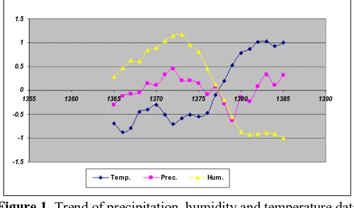
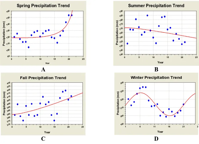
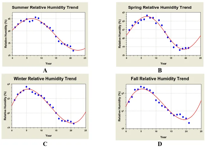
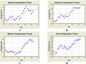
Data from five meteorological observatories in the selected stations were used in the analysis of climate change. The observed monthly and annual mean temperature, the estimated moving average and the observed values and trend of precipitation, humidity and temperature data were plotted for all stations and for regional analysis (Figures 1 to 3). These results indicate a statistical relationship between climate variability and temperature and can be used to estimate the impact of future climate variability. Precipitation did not show a significant trend (Figure 4 and Table 1). However, it showed a weak increase in annual time series. On the other hand, temperature parameters (Max, Min & Mean) showed increasing trends which was significant in 5% level where as the relative humidity showed a significantly decreasing trend (Figures 5 and 6 and Table 2). Figures 7 and 8 show the graphs for temperature trend assessment and Table 3 depicts the relevant modeling and its results.
-1.5 -1 -0.5 0 0.5 1 1.5
1355 1360 1365 1370 1375 1380 1385 1390
Temp. Prec. Hum .
Figure 1. Trend of precipitation, humidity and temperature data
0 200 400 600 800 1000 1200 1400 1600 1800 2000
1365 1370 1375 1380 1385 1390
لﺎﺳ
(
ر
ﺗ
ﻣﯾ
ﻠﯾﻣ
)
ﮫ
ﻧﻻ
ﺎﺳ
ط
ﺳ
و
ﺗﻣ
ﯽ
ﮔد
ﻧر
ﺎﺑ
Ramsar Noshahr Babolsar Qaem
Annual Precipitation Trend
Year P re c ipi ta ti o m ( m m )0 5 10 15 20 25
850 860 870 880 890 900 910 920 930 940
Figure 3. Modeling the annual precipitation trend
Spring Precipitation Trend
Year P re c ipi ta ti o n (m m )
0 5 10 15 20 25
90 100 110 120 130 140 150 160
Summer Precipitation Trend
Year P re c ipi ta ti o n (m m )
0 5 10 15 20 25
140 145 150 155 160 165 170 175 180 185 190
A B
Fall Precipitation Trend
Year P re c ip it a ti o n ( m m )
0 5 10 15 20 25
370 375 380 385 390 395 400 405 410 415 420 425 430
Winter Precipitation Trend
Year P re c ip it a ti o n ( m m )
1 6 11 16 21 26
190 200 210 220 230 240
C D
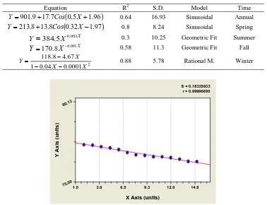
Table 1. The Model of Precipitation Trend Time Model S.D. R2 Equation Annual Sinusoidal 16.93 0.64
0.5 1.96
7 . 17 9 .
901
Cos X
Y
Spring Sinusoidal
8.24 0.8
0.32 1.97
8 . 13 8 .
213
Cos X
Y Summer Geometric Fit 10.25 0.3 X
X
Y
384
.
5
0.001Fall Geometric Fit 11.3 0.58 X X
Y 0.001
8 . 170 Winter Rational M. 5.78 0.88 2 0001 . 0 04 . 0 1 67 . 4 8 . 118 X X X Y
S = 0.18335933 r = 0.99996690
X Axis (units)
Y A x is ( u n it s )
1.0 3.8 6.5 9.3 12.0 14.8
75.00 90.13
Figure 5. Modeling the annual relative humidity trend
Table 2.The Model of Precipitation Trend
Time Model S.D. R2 Equation Annual Sinusoidal 0.15 0.99
0.23 1.44
1. 2 7 .
80
Cos X
Y
Spring Sinusoidal
0.25 0.97
0.25 1.7
9 . 1 6 .
80
Cos X
Y
Summer Sinusoidal
0.28 0.98
0.2 1.3
6. 2 4 .
79
Cos X
Y Fall Polynomial 0.28 0.96 3
2 0.002
09 . 0 8 . 0 5 .
81 X X X
Y
Winter Polynomial.
0.22 0.99
3
2 0.003
1 . 0 9 . 0
81 X X X
Summer Relative Humidity Trend
Year
R
e
la
ti
v
e
H
u
m
id
it
y
(
%
)
0 5 10 15 20 25
76 78 80 82
Spring Relative Humidity Trend
Year
R
e
la
ti
v
e
H
u
m
idi
ty
(
%
)
0 5 10 15 20 25
78 79 80 81 82 83
A B
Winter Relative Humidity Trend
Year
R
e
la
ti
v
e
H
u
m
id
it
y
(
%
)
0 5 10 15 20 25
78 80 82 84
Fall Relative Humidity Trend
Year
R
e
la
ti
v
e
H
u
m
id
it
y
(
%
)
0 5 10 15 20 25
79 81 83
C D
Figure 6. Modeling the seasonal relative humidity trend (A: Spring, B: Summer, C: Fall, D: Winter)
Annual Temperature Trend
Year
T
e
mp
e
ra
tu
re
(
C
)
0 5 10 15 20 25
15.8 16.3 16.8 17.3
Spring Temperature Trend Year T e m p e ra tu re ( C )
0 5 10 15 20 25
17 17 18 18 18 18 18 19
Summer Temperature Trend
Year T e m p e ra tu re ( C )
0 5 10 15 20 25
24.5 25.0 25.5 26.0 26.5 A B
Winter Temperature Trend
Year T e m p e ra tu re ( C )
0 5 10 15 20 25
7.5 8.0 8.5 9.0 9.5
Fall Temperature Trend
Year T e m p e ra tu re ( C )
0 5 10 15 20 25
14.6 14.8 15.0 15.2 15.4 15.6 15.8 16.0 16.2 16.4 C D
Figure 8. Modeling the seasonal temperature trend (A: Spring, B: Summer, C: Fall, D: Winter)
Table 3. The Model of Temperature Trend
Time Model S.D. R2 Equation Annual Sinusoidal 0.16 0.9 5 . 2 0005 . 0 9 . 1 1 . 18 X e
Y
Spring Sinusoidal 0.18 0.74 7 . 4 7 . 4 138971 3 . 18 2473680 X X Y Summer Sinusoidal 0.18 0.86 X e Y 24.7 0.003
Fall Polynomial 0.18 0.82 3 2 005 . 0 01 . 0 16 . 0 7 .
14 X X X
Y
Winter Polynomial. 0.22 0.88 2 003 . 0 17 . 0 1 15 . 1 5 . 8 X X X Y
compared with the mean temperature for the past 100 years (H. Yao, 1997).
In this paper, a hypothetical scenario of yearly increase of 0.06°C (1.2°C in last two decades) is showed by analyzing the temperature data in the study area. Temperatures in 2030 are given by T(N + 20, j) = AT(j) + 1.4, where Aj(j) is the total average of temperatures during N years (1800-2006) and y is the month number. Furthermore, it is assumed that the temperature rise would take place in a linear manner.
Stepwise regression equations for precipitation and temperature variables were not significant for Aug., Dec., Jan. and Feb. This was the same for humidity in Nov. and Feb. too. The results of stepwise regression method for humidity were better than precipitations.
The statistical relationship of temperature to other climatic factors was derived from long term data records and is assumed representative of the climate system of both present and future. It may be supposed that the climate system itself will not change dramatically under the global warming condition, and that the regression relationships can be used to estimate future conditions.
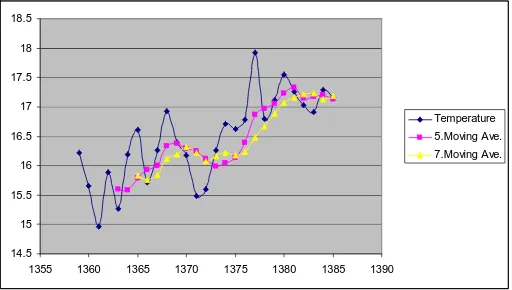
The results showed the increasing trend in mean annual temperature (0.06°C each year) and a decreasing trend for humidity simultaneous with temperature changes. Precipitation has a normal soft increasing trend in annul data (Figures 9 to 12). It can be claimed that precipitation changes had a regular variation in the last two decades and each yearit occurs around long mean precipitation value. So, increasing temperature and decreasing humidity are the effective parameters in regional climate changes in the study area.
14.5 15 15.5 16 16.5 17 17.5 18 18.5
1355 1360 1365 1370 1375 1380 1385 1390
Temperature
5.Moving Ave. 7.Moving Ave.
700 800 900 1000 1100 1200 1300 1400 1500
1355 1360 1365 1370 1375 1380 1385 1390
Precipitation
5.Moving Ave. 7.Moving Ave.
Figure 10. Mean annual precipitation observed and its trend
77 78 79 80 81 82 83 84 85 86
1355 1360 1365 1370 1375 1380 1385 1390
Humidity
5.Moving Ave.
7.Moving Ave.
Figure 11. Mean annual humidity observed and its trend
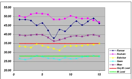
20.00 25.00 30.00 35.00 40.00 45.00 50.00 55.00
0 5 10 15
Ramsar Noshahr
Babolsar
Qaem Mean
Very M. Level
M. Level
Regarding the year 2030, a 20-year average temperature is produced from the assumed temperature series of 2021-2040. This value is then substituted into the regression formula and the corresponding average values for monthly precipitation, net radiation, humidity and wind speed were calculated and predicted respectively. These predicted values of 2021-2040 were compared with those of 1987-2006 which represent the present climate status; through which climate changes (in percentages) could be determined for the three sites. Usually there are five seasons in North of Iran: spring (March-April-May, MAM), rainy summer (June-July, JJ), hot summer (August-September, AS), autumn (October-November, ON) and winter (December- January-February, DJF).
4. Conclusion
There are two conclusive points about climate change results of this study. First, under the same scenario of future temperature rise, seasonal and annual climate at each site seems to change in a similar way. It may also mean that local climate responds to global warming and there are consistent regional trends. The results predicted that the potential evaporation increases seasonally and annually for all sites. The reason for this is that temperatures are estimated to become higher and humidity lower, both of which increase evaporative demand. Therefore, water demand would increase, which might result in more severe water supply conditions in future. However, we should note the De Martonne method results for climate index which showed no significant changes in the last three decades although temperature increased and relative humidity decreased. The amount of precipitation did not show significant changes but the precipitation systems has changed in the last two decades for winter precipitation (Snow to Rain) as a result of regional warming under influence of forest destruction and the increasing the CO2 concentration.
References
Adiku, S.G.K., and Stone, RC. 1995. Using the Southern Oscillation Index for improving rainfall prediction and agricultural water management in Ghana, Agricultural Water Management. 29 (1): 85-100.
Azizi, Q. 2000. El-nino and Dry/Wet periods of Iran, Journal of Geographic Research. 38: 71-84.
Bhalmc, H.P., Mooley, D.A., and Jabhav, S.K. 1983. Fluctuation in the Drought /flood areas over land and relationships with the Southern Oscillation.Monthly Weather Reverce. 111: 86-94.
Brad, B. 1994. Biospheric aspects of the hydrological cycle (BAHC), Focus 4: the weather generator project. HABC Report. 4: 2-12.
Chiew, F.H.S., Piechota, T.C., Dracup, J.A., and McMahon, T.A. 1998. El Nino/Southern Oscillation and Australian rainfall, stream flow and drought: Links and potential for forecasting Journal of Hydrology. 30: 138-149.
Dennett, M.D., Elston, J., and Prasad, P.C. 1978. Seasonal rainfall forecasting in Fiji and the Southern Oscillation. Agricultural Meteorology. 19 (1): 11-22.
EL-Askary, H., Sarkar, S., Chiu, L., Kafatos, M., El-Ghazawi, T. 2004. Rain gauge derived precipitation variability over Virginia and its relation with the El Nino southern oscillation, Advances in Space Research. 33 (3): 338-342.
Enslein, K., Ralston, A., and Wilf, H.S. 1977.Statistical Methods for Digital Computers. Wiley, New York, USA.
Haqshenas, A., Akhtari, R., and Saqafian, B. 2007. Investigating the effect of El-Nino and SOI on Floods of West south of Iran, Water and Waste water Journal. 18: 66-78. Hashino, M., and Yue, S. 1994.Statistical analysis of effects of monthly temperature on
monthly precipitation properties. In: Proc. Second Symposium on Earth Environment (Tokyo). 207-212. JSCE.
JMA.1990. Climate Changes as Greenhouse Gases Increase (In Japanese). Japan Meteorological Agency, Press of Ministry of Finance,Japan.
John, J., Oliver, J. E. 1993. Climatology an atmospheric science, New York, Macmillan Company. 169-178.
JUCH.W.R. 1995. Proc. Third PWRI- USGS Workshop on Hydrology, Water Resources and Global Climate Change.Japan-US Committee on Hydrology, Water Resources and Global Climate Change, Tuskuba, Japan.
JUCH, W.R. 1992. Proc. Workshop on the Effects of Global Climate Change on Hydrology and Water Resources at the Catchment Scale.Japan-US Committee on Hydrology, Water Resources and Global Climate Change, Tuskuba, Japan.
Khoshakhlaq, F. 1998. ENSO and its effect on Precipitation regime of Iran, Geographic Research Journal. 51:78-89.
Linacre, E.T., and Geerts, B. 1997. Climates and weather explained, London, Routledge. 432 pp.
Lucero, O.A. 1998. Effects of the southern oscillation on the probability for climatic categories of monthly rainfall, in a semi-arid region in the southern mid-latitudes, Atmospheric Research. 49: 337-348.
Modarres poor, A. 1996. ENSO and Abnormality in Clima of Iran, Msc. thesis, Islamic Azad University. 189 pp.
Nazem, Al Sadat, S.M., and Qasemi, A.R. 2003. ENSO and Precipitation of cold 6-months of Central and West South of Iran, Agricultural and Natural Resources Technology. 7:1-13. Nazem Al Sadat, S.M., Rahimi, M., andKeshavarzi, A. 2006.b. Assessment of ENSO
effective on Hydrological condition of rivers in Fars Province in Dry/Wet Periods, Journal of Iranian Agricultural Science. 37: 361-369.
Nazem Al Sadat, S.M., Samani, N., Yari, A., Molaei., and Nikoo, M. 2005. ENSO and Climate change and Precipitation Variations in South and West South of Iran, Scientific Journal of Agriculture. 28: 81-100.
Nazem Al Sadat, S.M. 1999. Investigation on El-nino and southern oscillations effective on Fall Precipitation of Iran, Second Regional Conference of Climate Change, Meteorological Organization of Iran.
Paeth, H., Anja, S., Petra, F., and Andreas, H. 2008. Uncertainties in climate change prediction: El Niño-Southern Oscillation and monsoons, Global and Planetary Change. 60 (3-4): 265-288.
Qayour, A., and Asakere, H. 2001. Study of Remote Sensing effects on Iran Climatology. Geographic Research Journal. 64: 93-113.
Quinn, W.H. 1992. A study of the Southern Oscillation- related climatic activity for A.D. 622-1900 incorporating Nile flood data in El Nino: Historical and paleoclimatic aspects of the southern oscillation, edited by M.H. Glantz, New York, Cambridge University Press. pp.119-648.
Quinn, W.N., Zopf, D.O., Short, K.S., and KuoYnag, R.T. 1978. Historical trends and statistics of the southern Oscillation, El NiNo and Indonesian droughts, Fishery Bulletin. 76: 663-678.
Ranatunge, E., Malmgren, B.A., Hayashi, Y., Mikami, T., Morishima, W., Yokozawa, M., and Nishimori, M. 2003.Changes in the Southwest Monsoon mean daily rainfall intensity in Sri Lanka: relationship to the El Niño–Southern, Palaeogeography, Palaeoclimatology, Palaeoecology. 197(1-2): 1-14.
Rasmusscn, E.M., and Carpenter, T.H. 1983. The relationship between eastern equatorial Pacific Sea surface temperatures and rainfall over Indian and Srilanka, Monthly Weather Reverse. 111: 517-528.
Rasmusson, E.M., and Wallace, J.M. 1983. Meteorological aspects of the El Nino / southern oscillation. Science. 222: 1195-1202.
Ropelewski, C., and Halpert, M. 1987. Global and regional scale precipitation patterns associated with El Nino / Southern oscillation, Monthly Weather Reverse. 115: 2352-2362.
Streten, N.A. 1983. Southern hemisphere circulation contrasts in the winter 1972 and 1973. Preprint first international conference on the southern hemisphere meteorology, Sao Joase das Capos, Brazil. pp. 108-111.
Suppiah, R. 1988. Atmospheric circulation variations and the rainfall of Serilanka, Science. Rept., Inst. Geoscience, University of Tsukuba, 9: 75-142.
Tyson, P.D. 1987. Climatic change and variability in Southern Africa, Cape Town, Oxford University Press.
Walker, G.T. 1923. Correlation in seasonal variations of weather, VIII: A preliminary study of world weather, Indian Meteorology Department. 24: 75-131.
Walker, G.T. 1924. Correlation in seasonal variations of weather, IX: A further study of world weather, Royal Meteorology Society. 3: 81-95.
Walker, G.T. 1928. World weather III: Royal Meteorology Society. 2: 97-104.
Whetton, P., and Rutherford, I. 1994. Historical ENSO tele connections in the Eastern Hemisphere, Climate changes. 28: 221-253.
Yao, H., Terakawa, A., and Hashino, M. 1997. Predicting future changes in climate and evaporation by stepwise regression method. Sustainability of water resources under increasing uncertainty, IAHS Publication. 24: 273-288.