S
c
h
o
o
l
o
f
E
c
o
n
o
m
ic
s
&
F
in
a
n
c
e
D
is
c
u
s
s
io
n
P
a
p
e
r
s
Procedures for Eliciting Time
Preferences
David Freeman, Paola Manzini, Marco Mariotti and Luigi Mittone
School of Economics and Finance Discussion Paper No. 1513 20 Oct 2015
Procedures for Eliciting Time Preferences
David Freeman
⇤Simon Fraser University
Paola Manzini
University of St. Andrews and IZA
Marco Mariotti
Queen Mary University of London
Luigi Mittone
University of Trento
This version: October 2015
Abstract
We study three procedures to elicit attitudes towards delayed payments: the Becker-DeGroot-Marschak procedure; the second price auction; and the multiple
price list. The payment mechanisms associated with these methods are widely considered as incentive compatible, thus if preferences satisfy Procedure Invariance, which is also widely (and often implicitly) assumed, they should yield identical
time preference distributions. We find instead that the monetary discount rates elicited using the Becker-DeGroot-Marschak procedure are significantly lower than
those elicited with a multiple price list. We show that the behavior we observe is consistent with an existing psychological explanation of preference reversals.
J.E.L. codes: C91, D9
Keywords: time preferences, elicitation methods, Becker-DeGroot-Marschak pro-cedure, auctions, multiple price list.
∗We wish to thank all the tireless staff at CEEL, and in particular Marco Tecilla, for the excellent
1
Introduction
Incentivized experiments that study choices among delayed rewards have been widely used to measure and test hypotheses about time preferences. Several elicitation methods have been viewed as “incentive compatible” means of eliciting precise information about time preferences. Three such procedures have become workhorse methods in experimental economics, psychology, and neuroeconomics: the multiple price list (MPL), the Becker, DeGroot, and Marschak [3] procedure (BDM), and the second price auction (SPA).1
We study the MPL, the BDM, and the SPA as procedures for eliciting preferences over delayed payments. The MPL is a choice task, in that subjects have to choose be-tween a smaller-sooner and larger-later pair of outcomes. BDM and SPA are instead both instances of matching tasks, in which subjects name a ‘sooner’ amount they regard as indifferent to a later fixed reward. Regardless of these aspects, if the payment mecha-nism associated with each method is incentive compatible and subjects have preferences over delayed rewards that are invariant to the procedure by which they are elicited, we ought to recover the same distribution of time preferences from each method. With few exceptions, economic experiments using these three methods draw an interpretation of subjects’ behavior that implicitly assumesIncentive Compatibility of the payment mecha-nism andProcedure Invariance of subject preferences. In this paper we instead treat these assumptions as testable, and we test their implications using a between-subject design.
Previous work in experimental economics has noted systematic differences in the rank-ings of lotteries inferred from their monetary valuations elicited using the BDM as com-pared to direct choices in choice tasks (e.g. Grether and Plott [13]). However, this literature on ‘preference reversals’ has focused on choice under risk. To the best of our knowledge, there is no existing incentivized study that indicates whether analogous prefer-ence reversals occur in intertemporal choice. A leading economic explanation of preferprefer-ence reversals under risk is based on the interaction between the random component of the pay-ment mechanism, the risky alternatives, and a failure of the Independence Axiom (e.g. Karni and Safra [20]). But such an explanation is highly specific to choice under risk: there is no compelling reason to expect analogous preference reversals in intertemporal choice. On the other hand, existing work that compares different experimental techniques
1
for studying time preferences does not use any incentives (Tversky et al. [28] Study 2; Read and Roelofsma [24]; Hardisty et al. [14]), and thus do not offer direct information about economic choices.
We find a significant difference in subject responses between the MPL and BDM. This is in spite of an implementation ensuring that a subject in each procedure faced exactly the same economic incentives. The direction of this effect is consistent with Tversky et al.’s [27] scale compatibility hypothesis, which hypothesizes that a subject responding with a monetary amount in a matching task like BDM will put more weight on monetary outcomes than in a comparable choice task like the MPL.
The paper is organized as follows. Section 2 describes our experimental design. In Section 3 we lay out Incentive Compatibility and Procedure Invariance as testable assump-tions, we discuss their implications for our experiment, and we review the predictions of existing economic and psychological explanations of preference reversals for our experi-ment. We present our results in Section 4 and we discuss them in Section 5.
2
Experimental design
Our experiment implements a between-subjects design to study three procedures – the MPL, BDM, and SPA – for eliciting each subject’s preferences between sooner payments and a fixed later payment.
We ran four sessions for each of the three treatments, with 16 inexperienced subjects per session between June 2012 and March 2013. Subjects for each session were recruited from the CEEL database at Universit`a di Trento. All subjects received ae5 participation
payment at the end of the session on top of any payments based on their choices. Each subject could only participate in one treatment of the experiment. An average session lasted less than 45 minutes, and the average subject payment was e14.40.
The subjects were given instructions that explained the task they would face and how they would be paid based on their choices. Then they completed a comprehension test on the instructions.2 In each treatment, we use a single elicitation procedure (MPL,
BDM, or SPA) to elicit the monetary amount paid tomorrow that would be indifferent to the receipt of a e20 at each of three possible delays (1, 2 and 4 months) for each
subject. We implemented this by presenting subjects with a screen with three buttons,
2
each corresponding to one of the time horizons. Subjects could enter money amounts in e0.50 increments in all treatments. To avoid any order effects, subjects were free to
choose the order in which to tackle each task. After completing each choice task, subjects were sent back to this screen with the buttons corresponding to the time horizons already completed appearing greyed out.
In order to incentivize subjects to report their economic preferences, 50% of the sub-jects in each group were drawn at random to receive a payment based on their choices. At the end of the experiment we drew from a uniform distribution which 8 subjects (out of 16 participants in each computerized session) would receive a payment in addition to the show up fee; which screen (1 month, 2 months or 4 month delay) would ‘count’, and, in the case of the MPL or BDM elicitation method, which row or monetary amount would be drawn to determine their payment.
In the second part of the experiment, we test the subjects’ awareness of the interest rates implied by their previous choices3 and measure their personality traits. This part
of the experiment was common across all treatments; we discuss these results in the Appendix.
2.1
Multiple Price List
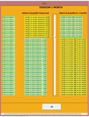
In each row of our MPL, a subject chooses between Option A – an amount paid tomorrow that varies betweene20 in the first row and decreases toe0.50 in the last row – and Option
B, which gives e20 at the later date corresponding to the task. In our implementation
of the MPL, we enforce a single switching line in each list by having the subject move a slider down the screen to indicate the rows in which she chooses Option A.
2.2
Becker-DeGroot-Marshack
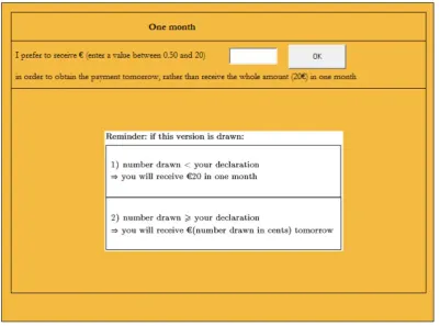
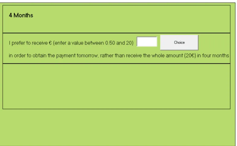
Participants in the BDM treatment were asked in each of the three tasks to state the lowest amount L that they would prefer to receive tomorrow instead of receiving e20 at
the later date corresponding to that task. For each of the three time horizons, if the value declared was not larger than a value drawn from a uniform distribution with support
3
After all values have been elicited, subjects are asked to state the three annual (non-compound)
interest rates that correspond to their choices in each time horizon. For instance, a declaration of e19
in the four month horizon question would have implied an annual interest rate of 15.75%. Subjects were
instructed that they would be remunerated ate2 ore1 depending on whether the answer was within a
on {e0.5,e1, . . . ,e20}, then the subject would receive a payment equal to the number
drawn the following day; otherwise she would get the full amounteL with delay.
2.3
Second Price Auction
As in the BDM treatment, participants in the SPA treatment were asked in each of the three tasks to state the lowest amount Lfor which they would prefer to receive tomorrow instead of receiving e20 at the later date corresponding to that task. For each of the
three time horizons, when a subject was paid based on that auction task, if they had the lowest bid they received tomorrow the second-lowest stated amount stated by all subjects; otherwise they receivede20 at the later date. The outcome of each auction was
not revealed before the next auction was played, as in our other treatments.
3
Eliciting Time Preferences: Theory
3.1
Payment Mechanisms, Procedure Invariance, and Eventwise
Monotonicity
For a subject who makes a single pairwise choice, the interpretation of this choice is uncontroversial from the perspective of standard economic theory: it defines her preference between two options. However, a single pairwise choice only provides limited information about a subject’s preferences.
For this reason, past work has used the MPL, BDM, and SPA procedures to elicit finer information about the entire preference relation on the domain of interest. However, the validity of each method for eliciting preferences relies on some crucial assumptions.
First, preferences cannot depend on economically irrelevant features of the procedure that is used to elicit them – this is the Procedure Invariance assumption. While such an invariance is almost universally assumed, often implicitly so, it is testable. Second, any experiment that attempts to make multiple observations of a subject’s preference relation must decide how multiple choices (that is, preference statements) determine a payment at the end of the experiment. Depending on how a subject’s payment is determined from her portfolio of implied preference statements, she may or may not wish to report her true preferences. Which is the case will be driven by her preference over portfolios, given the experiment’s payment mechanism.
and let T ={1 day, 1 month,2 months,4 months} denote a set of payment dates. In the standard economic approach to decision-making (e.g. Fishburn and Rubinstein [10]), a subject has a single transitive preference relation % over dated rewards in M ⇥T, and this preference is procedure invariant, as explained above. The Monetary Monotonicity
property requires that subjects prefer more money to less given a fixed horizon. Formally,
% satisfies Monetary Monotonicity if for any m, m0 2M, m > m0 implies (m, t)$(m0, t) for any t2T.
In our implementation of the MPL, such a subject makes a choice in each row of the MPL, which determines a smallest value mM P L 2 M for which the subject picks
!
mM P L,t,1 day"
over (e20, t). In our implementations of the BDM and SPA, a subject
is asked to state an amount mi,t (i 2 {BDM,SPA}) for each of t = 1m,2m,4m. With
; denoting exclusion from payment, the payment mechanism corresponding to procedure
i picks a state ! 2 M ⇥ {1m,2m,4m} [ {;} that determines a subject’s payment given her announcements {mi,1m, mi,2m, mi,4m}. When the mechanism determines state !, a subject in procedure i declaring {mi,1m, mi,2m, mi,4m} receives a payment determined byφi : Ω!M ⇥T [ {(0,now)}given by
φi(!) =
8 > > > < > > > :
(0,now) if !=;
(m, t) if != (m, t) and m > mi,t
(mi,t,1 day) if != (m, t) and mmi,t
for alli2 {MPL,BDM,SPA}. Each payment mechanism is a Savage act4 φi over delayed payments in M ⇥T.
We wish to interpret a report of mi,t as implying the preference statements (m, t) $ (e20, t)$(m0, t) for anym, m0 2M satisfying m > mi,t > m0. Since our payment mech-anism is a Savage act, whether a subject’s report admits such an interpretation depends on her preferences over acts. As shown in Azrieli et al. [1], such an interpretation will be appropriate if the subject has transitive preferences over M ⇥T that satisfy Mone-tary Monotonicity and an additional property calledEventwise Monotonicity. Intuitively, Eventwise Monotonicity holds whenever an act that yields more preferred dated rewards in each state as compared to another is also ranked higher by the preference over Savage acts. Formally, given a subject’s transitive preference relation over dated rewards %, a subject’s preference relation %? on Savage acts satisfies Eventwise Monotonicity if, for any two acts f and g, f(!)%g(!) for all ! 2Ω implies that f %? g, and if f(!)%g(!)
4
for all ! 2Ω andf(!)$g(!) for at least one !2Ω , then f $? g.5
Our discussion of the implications of properties of preferences for the incentive compati-bility of experimental methods is summarized in the observation below.
Observation. 1. If a subject has Procedure Invariant preferences %? on Savage acts over M ⇥ T that satisfy Eventwise Monotonicity, then each subject would an-nounce the same value mi,t in each procedure i 2 {MPL,BDM,SPA} given the horizon
t 2 {1 month,2 months,4 months}. If a subject’s preferences % on M ⇥T also satisfy Monetary Monotonicity, then for any horizon t 2 {1 month,2 months,4 months}, pro-cedure i 2 {MPL,BDM,SPA}, and amounts m, m0 2 M with m > mi,t > m0, we have (m, t)$(e20, t)$(m0, t).
2. If a subject would announce different values mBDM,t 6=mMPL,t for some horizon
t 2 {1 month,2 months,4 months}, then this subject cannot have Procedure Invariant preferences on Savage acts over M ⇥T. If a subject would announce values mSPA,t 6=
mMPL,t or mSPA,t 6= mBDM,t for some horizon t 2 {1 month,2 months,4 months}, then this subject cannot have preferences on Savage acts over M ⇥T that satisfy both Procedure Invariance and Eventwise Monotonicity.
3.2
Alternative Hypotheses
Incentives. Economic theories that maintain the existence of procedure invariant eco-nomic preferences have posited that the payment mechanism could be responsible for preference reversals in BDM in the domain of choice under risk (Karni and Safra [20]), violating Eventwise Monotonicity.6 Karni and Safra’s theory relies on the fact that in
choice under risk, a subject’s choices combined with a random problem selection mecha-nism with objectively given probabilities determines a compound lottery; a subject who reduces compound lotteries will only want to report their preferences over lotteries if she has expected utility preferences. In the domain of delayed payments, none of our payment mechanisms forms a compound lottery and there is no obvious analogue of re-duction. Thus we see no compelling reason why incentives ought to generate differences across treatments according to Karni’s and Safra’s theory. Moreover, since the exact same objectively-given randomization process is used in MPL and BDM mechanisms, according
5
The mechanisms we study fall into the class of Random Problem Selection mechanisms in Azrieli et al. [1]. They show that Eventwise Monotonicity is a sufficient, and ‘almost’ necessary condition for
each Random Problem Selection mechanism to correctly elicit % – or in other words, to be incentive
compatible. The discussion leading to their Theorem 1 provides details.
6
to this theory there is no possibility of incentive-driven preference reversals between the MPL and BDM treatments.
Response mode. The MPL has a subject respond with her row-by-row choices (a choice task), while the BDM and SPA ask a subject to state a monetary amount to a later payment that would make her indifferent between the sooner monetary amount and a e20 later payment (matching tasks). Tversky et al. [27] argue that the response mode
can affect the weight that a decision-maker places on each of multiple attributes, which is inconsistent with procedure invariant economic preferences. Their scale compatibility hypothesis posits that subjects in matching tasks will put more weight on the matched attribute - in our case, the monetary payment. This hypothesis can correctly predict the pattern of commonly observed preference reversals over risk following Grether and Plott. Tversky et al. [27] find some evidence to support their hypothesis when comparing choice and matching tasks involving purely hypothetical delayed rewards. Their hypothesis predicts thatmM P L,t < mBDM,t=mSP A,t for any subject.
Confusion in BDM. Cason and Plott [4] hypothesize that many subjects incorrectly believe that they will receive the payment stated in the BDM should a “winning” num-ber be drawn; akin to misperceiving that φBDM((m, t)) = !
mBDM,t, t" whenever m ≥
mBDM,t.7 If preference %? satisfies Eventwise Monotonicity but a subject misperceives
φBDM as such, she would pick mBDM,t > mM P L,t. However, Cason and Plott are silent on how subjects would behave in a SPA against human bidders with nearly identical instructions.
Biases in Auctions. Previous research has documented a bias towards overbidding one’s value in second price auctions with induced private values (Kagel and Levin [18]) and also with private homegrown values (as compared to bids in BDM; Rutstr¨om [25]). One hypothesis is that this arises due to a desire to win in a competitive environment. In our experiment, this would lead to lower bids in the SPA treatment.
7
4
Results
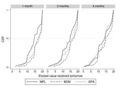
We find that subjects’ responses are consistently the lowest in the MPL and highest in the BDM (Table 1, Figure 1).
MPL BDM SPA
One month Mean 14.77 16.83 16.39
Median 15.00 18.00 18.00
Two months Mean 14.17 16.30 15.23
Median 15.00 17.25 16.50
Four months Mean 13.58 15.03 13.79
Median 14.50 15.00 15.00
[image:10.595.164.436.152.292.2]Sample size 64 64 64
Table 1: Elicited values by treatment
0
.5
1
0 5 10 15 20 0 5 10 15 20 0 5 10 15 20
1 month 2 months 4 months
MPL BDM SPA
CDF
Elicited value received tomorrow
Figure 1: Distribution of elicited values by treatment
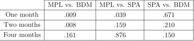
[image:10.595.105.499.357.644.2]MPL vs. BDM MPL vs. SPA SPA vs. BDM
One month .009 .039 .671
Two months .008 .159 .210
Four months .161 .876 .150
[image:11.595.131.468.72.144.2]Two-sided p-values for rank-sum test of equality of distribution.
Table 2: Tests of equality of responses across treatments
of the three horizons at the 5% significance level (Table 2). The responses between the SPA and BDM do not statistically differ on any horizon (at the 10% level), and only on the one month horizon do the distribution of responses in the SPA and MPL differ statistically at the 5% significance level. Figure 1 shows that differences across treatments are systematic across horizons and throughout the distribution.
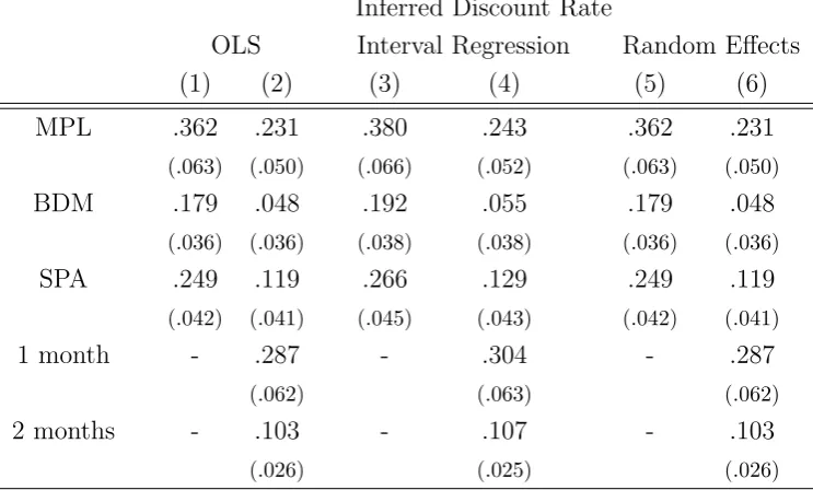
We use regression techniques to conveniently summarize how inferred monetary dis-count rates differ across treatments.8 We wish to estimate the regression equation:
rit=⇢MM P Li+⇢BBDMi+⇢ASP Ai+Xitβ+✏it
The variablerit denotes the monthly monetary discount rate inferred (under the assump-tions of Monetary Monotonicity and Eventwise Monotonicity) from subject i’s behavior in horizont,M P L, BDM, SP A are treatment dummies, Xit denotes additional controls, and✏ denotes an error term. However, even under these assumptions our treatments only measure an interval forrit giveni’s response in horizont. In specifications 3 and 4 (Table 3), we use interval regressions to account for this under the assumption that the ✏it are independently and normally distributed. Specification 3 includes no control variables in
X, while specification 4 includes time horizon dummies to account for the possibility of non-constant discounting over monetary amounts. We assume that discount rates are weakly positive; thus values of rit are bounded below by 0 and the empirical distribution of rit is rightly skewed with a mode close to 0. For this reason, the normality assumption embedded in the interval regression is highly inappropriate for our data.9 In specifications
1, 2, 5, and 6 we use least squares estimators with the minimum of the inferred interval
8
Our inferred monetary discount rates measure do not account for the possibility that individuals discount their utility of payments and have a curved money function. A subject’s utility-for-money function is not separately identified from her discount rate on our domain, even if we assumed power utility-for-money functions. This mechanically implies that the inferred discount rates here will exceed that of studies that work with a curved utility-for-money function.
9
We note that an application of interval regression based on an asymmetric distribution for✏it might
Inferred Discount Rate
OLS Interval Regression Random Effects
(1) (2) (3) (4) (5) (6)
MPL .362 .231 .380 .243 .362 .231
(.063) (.050) (.066) (.052) (.063) (.050)
BDM .179 .048 .192 .055 .179 .048
(.036) (.036) (.038) (.038) (.036) (.036)
SPA .249 .119 .266 .129 .249 .119
(.042) (.041) (.045) (.043) (.042) (.041)
1 month - .287 - .304 - .287
(.062) (.063) (.062)
2 months - .103 - .107 - .103
(.026) (.025) (.026)
Robust standard errors clustered at the subject level in brackets.
[image:12.595.113.485.77.301.2]Random effects coefficients and standard errors computed using lincom in Stata.
Table 3: Inferred discount rates by treatment
of discount rates as the left-hand side variable as checks on the robustness of the interval regression.10 We use ordinary least squares to estimate in specifications 1 and 2 to
esti-mate the same regression equations as 3 and 4. To account for individual heterogeneity, we add an individual-specific dummy to specifications 1 and 2, and estimate the resulting model using a generalized least squares random effects estimator (specifications 5 and 6). We obtain similar results across specifications (Table 3). Focusing on our results from the interval regression (specification 3), the inferred monetary discount rate is highest in the MPL (.380), lowest in the BDM (.192), and intermediate in the SPA (.266). The difference between the MPL and BDM is statistically significant (p=.01) but the differ-ence between the MPL and SPA is not (p=.15), nor is the difference between the BDM and SPA (p=.20). We obtain qualitatively and quantitatively similar results using both ordinary least squares and generalized least squares random effects with the minimum of the inferred interval of discount rates as the left-hand side variable, and also if we include time horizon dummy variables to account for non-constant monetary discount rates. In each specification in Table 3, the inferred discount rate is on average .18-.19 higher in the
10
There were only three times when a subject chose e0.50 tomorrow over the more delayed e20, but
MPL than in the BDM, a significant difference at the 5% level, while the inferred average discount rates in the SPA treatments do not significantly differ from either of the other two treatments.
5
Discussion
We found evidence of a substantial difference in the discount rates inferred from subjects in the MPL as compared to the BDM. Since these elicitation schemes have the same incentive structure, this difference violates Procedure Invariance. The direction of this bias – towards more inferred patience in the BDM – is consistent with Tversky et al.’s [27] scale compatibility hypothesis. It is also consistent with Cason and Plott’s [4] conjecture that many subjects systematically misperceive the BDM, and believe that they receive their stated amount should the BDM draw an amount that exceeds it.
Since there are systematic albeit statistically insignificant differences between behavior in the SPA and the other two methods, we view these differences as merely suggestive. We note that Cason and Plott do not state whether an analogous mistake ought to occur in an SPA setting with multiple human bidders. In our context we see such an extension as natural. Such a mistake, however, would (counterfactually) predict underbidding in private value SPAs. In contrast, the conjunction of the scale compatibility hypothesis and a previously documented bias towards making winning bids in auctions could explain why bids in the SPA tend to be higher than in those in the BDM.
Our discussion has taken the MPL as a benchmark. Findings from past intertemporal choice experiments that use the MPL have not provided evidence of any inconsistency with the combination of Eventwise Monotonicity and Procedure Invariance (Andersen et al. [2]). The existing evidence from choice under risk that is inconsistent with the combination of Eventwise Monotonicity and Procedure Invariance can be explained by the incentive scheme (i.e. a failure of Eventwise Monotonicity; Freeman et al. [12]) – unlike the results here.
for informal loans in Bangalore, India (Kalkod [19]) and annualized interest rates in the 279-1199% range on payday loans in British Columbia, Canada.11
We believe that the evidence we have provided demonstrates the potential value of incorporating context-dependence into economic theories of intertemporal choice (like that of Tversky et al. [27]). Such models could be particularly valuable for analyzing the results of economic experiments. We submit that, if our goal is to use economic experiments to better understand real world decisions, future experimental work on the elicitation of “time preferences” should treat context-dependence as a variable of interest rather than an issue to be ignored or treated as a confound.
References
[1] Azrieli, Y., C. Chambers and P.J. Healy (2015). Incentives in Experiments: A The-oretical Analysis. Working paper. 3.1, 5
[2] Andersen, S., G. W. Harrison, M. I. Lau and E. E. Rutstr¨om (2006) “Elicitation using multiple price list formats”, Experimental Economics, 9: 383-405. 5
[3] Becker, G. M., M. H. DeGroot, and J. Marschak (1964). “Measuring utility by a single-response sequential method”,Behavioral Science, 9(3): 226-232. 1
[4] Cason, T.N., and C. R. Plott (2014). “Misconceptions and Game Form Recognition: Challenges to Theories of Revealed Preference and Framing”, Journal of Political Economy, 122(6): 1235-1270. 3.2, 5
[5] Coller, M. and M. Williams (1999). “Eliciting Individual Discount Rates”, Experi-mental Economics, 2(2): 107-127. 1
[6] Cooper, N., J. Kable, B.K. Kim, G. Zauberman (2013). “Brain activity in valuation regions while thinking about the future predicts individual discount rates.” Journal of Neuroscience, 33(32): 13150-13156. 1
[7] Cox, J. and S. Epstein (1989). “Preference reversals without the independence ax-iom.” American Economic Review,79(3): 408-426. 6
[8] Dohmen, Thomas, Armin Falk, David Huffman and Uwe Sunde (2012). “Interpret-ing Time Horizon Effects in Inter-Temporal Choice,” IZA Discussion Papers 6385, Institute for the Study of Labor (IZA). 1
11
[9] Filiz-Ozbay, Emel, Jonathan Guryan, Kyle Hyndman, Melissa Kearney, Erkut Ozbay (2015). “Do Lottery Payments induce savings behavior? Evidence from the Lab.”
Journal of Public Economics 126: 1-24. 1
[10] Fishburn, P. C., and A. Rubinstein (1982). ”Time preference.” International Eco-nomic Review, 23(2): 677-694. 3.1
[11] Frederick, S., G. Loewenstein and T. O’Donoghue (2002). “Time discounting and time preferences: a critical review”, Journal of Economic Literature, vol. 40: 351-401. 5
[12] Freeman, D., Y. Halevy, and T. Kneeland (2015). “Eliciting Risk Preferences Using Choice Lists”, Working Paper. 5
[13] Grether, D.M., and C.R. Plot. (1979). “Economic theory of choice and the preference reversal phenomenon”, American Economic Review, 69(4): 623-638. 1
[14] Hardisty, David J., Katherine F. Thompson, David H. Krantz and Elke U. Weber (2013). “How to measure time preferences: An experimental comparison of three methods”, Judgment and Decision Making, 8 (3): 236-249. 1
[15] Harrison, G., M. Lau and M. Williams (2002). “Estimating Individual Discount Rates in Denmark: A Field Experiment.” American Economic Review 92(5): 1606-1617. 1
[16] Horowitz, J. K. (1991). “Discounting money payoffs: an experimental analysis”, in S. Kaish and B. Gilad (Eds.),Handbook of Behavioral Economics (vol 2B, pp. 309-324), Greenwich, CT, JAI Press. 1
[17] Ifcher, J. and H. Zarghamee (2011). “Happiness and time preference: the effect of positive affect in a random-assignment experiment.” American Economic Review
101(7): 3109-3129. 1
[18] Kagel, J.H., and D. Levin (1993). ”Independent private value auctions: Bidder be-haviour in first-, second-and third-price auctions with varying numbers of bidders”,
Economic Journal, 103(419): 868-879. 3.2
[19] Kalkod, R (2011). “Violence rules money-lending rackets”, Times of India, October 4, 2011. 5
[21] Kirby, K. N. (1997). “Bidding on the future: Evidence against normative discounting of delayed rewards”, Journal of Experimental Psychology: General, 126: 54-70. 1
[22] Lee, K. and M. C. Ashton (2008). “The HEXACO Personality Factors in the Indige-nous Personality Lexicons of English and 11 Other Languages”, Journal of Person-ality, 76: 1001-1054. C, C.1
[23] Plott, C. R., and K. Zeiler (2005). “The Willingness to Pay–Willingness to Accept Gap, the ‘Endowment Effect’, Subject Misconceptions, and Experimental Procedures for Eliciting Valuations”, American Economic Review, 95(3): 530-545.
[24] Read, D. and R. Roelofsma (2003). “Subadditive versus hyperbolic discounting: A comparison of choice and matching”, Organizational Behavior and Human Decision Processes, 91(2): 140-153. 1
[25] Rutstr¨om, E. (1998). “Home-grown values and incentive compatible auction design”,
International Journal of Game Theory, 27(3): 427-441. 3.2
[26] Savage, L. J. (1954). The Foundations of Statistics. John Wiley & Sons, New York, NY 4
[27] Tversky, A. , S. Sattath and P. Slovic (1988). “Contingent weighting in judgment and choice”, Psychological Review, 95(3): 371-384. 1, 3.2, 5
[28] Tversky, A., P. Slovic, and D. Kahneman (1990). ”The causes of preference reversal”,
American Economic Review,80(1): 204-217. 1, 6
Appendices
A
Instructions
The translation of the original instructions (in Italian) follows below (we omit the com-prehension test for space reasons - it showed three screens, one for each time horizon, as filled by an hypothetical participants. On each screen two simple questions asked about what payment would the hypothetical participant received if drawn or not drawn. Links to screenshots and our experimental software is available here.
A.1
Sheet 1 (common to all treatments)
This experiment studies choice over time. Please read carefully the instructions that follow while an assistant also reads them aloud. You will be given a fixed participation fee at the end of the experiment. Moreover you may be able to receive an additional sum on top of the participation fee. This additional amount will depend on your choices and on a random draw. More precisely, you will have one chance in two to be drawn to receive the additional payment.
At the end of the experiment we will ask you to complete a questionnaire. The information collected will be used solely for research purposes. The information collected will be kept completely anonymously.
Click ‘NEXT’ to continue.
A.2
Sheet 2
A.2.1 MPL
TAKING PART IN THE EXPERIMENT
Option A instead is different on all rows, and varies between a minimum of e0.50 and a
maximum of e20. Careful! You must make a choice in each row. To do so you will have
to use the cursor in the middle of the screen: you can scroll it using the mouse to select the option that you prefer in each row. You will see three tables in total, differing from one another only for the delay with which thee20 of option B are payable.
Three random draws will take place at the end of the experiment. The first will draw one of the three screens, the second will draw one of the forty rows from that screen, and the third will draw the participants which will receive the additional payment, corresponding to the choice made in the row drawn. This means that if you are drawn to receive a payment, the amount of money you will receive will be that corresponding to the option (A or B) that you chose in the row drawn. This means that each choice you will make in each of the three tables may be rewarded.
Click ‘NEXT’ to continue
A.2.2 BDM
TAKING PART IN THE EXPERIMENT
By participating in this experiment you have one chance in two of being drawn to receivee20, which will be payable with a delay of some weeks. However you will have the
opportunity to anticipate receipt to tomorrow. In this case you will have to give up part of the total amount. Very shortly you will see a screen where you will be able to declare the minimum amount you are prepared to receive in place of the fulle20 to receive your
payment tomorrow, entering a value between e0.50 and e20 in e0.50 steps. After your
choice a number between e0.50 and e20 in e0.50 increments will be drawn at random.
Every value betweene0.50 ande20 ine0.50 increments has the same probability of being
drawn
How much is the early payment?
If you are drawn for payment:
1) if your declared value smaller or equal to the one drawn, you will be entitled to receive tomorrow an amount of money equal to the number drawn.
2) if your declared value is larger than the one drawn, you will be entitled to the full
e20 but with delay.
How much to declare?
If you think about it, you will see that the best option for you is to declare the amount that makes you indifferent between receiving such amount tomorrow or the whole e20
declaree0.50, you will be sure that, if drawn for payment, you will receive your payment
tomorrow, but you could earn as little as e0.50 in case the number drawn is e0.50. If
you declare e20 you will be sure that, if drawn for payment, you will receive the whole e20 albeit with delay: the exception is if e20 is drawn, in which you would receive e20
tomorrow. Yet even in this case if the declaration which makes you indifferent is less than
e20, by declaring such value you would receive e20 tomorrow anyway.
You will be shown three screens in total, which differ only for the delay with which the full e20 are payable.
Three random draws will take place at the end of the experiment. The first will draw one of the three screens, the second will draw a number between e0.50 and e20 in e0.50 increments, and the third will draw the participants who will receive a payment
corresponding to the choices made. This means that if you are drawn to receive a payment, the amount of money you will receive will be based on the choice you made in the screen drawn. This means that each choice you will make in each of the three screens may be rewarded.
Click ‘NEXT’ to continue
A.2.3 SPA
TAKING PART IN THE EXPERIMENT
By participating in this experiment you have one chance in two of being drawn to receive e20, which will be payable with a delay of some weeks. However you will have
the opportunity to anticipate receipt to tomorrow. In this case you will have to give up part of the total amount. Very shortly you will see a screen where you will be able to take part in an auction to anticipate the payment to tomorrow. As the other participants, you will have to declare the minimum amount you are prepared to receive in place of the full e20 to receive your payment tomorrow, entering a value between e0.50 and e20 in e0.50 steps. The participant declaring the lowest value will acquire the right to receive
the payment earlier. If two or more participants have inserted the same minimum value, all of these participants will acquire the right to receive the payment earlier.
How much is the early payment?
If you are drawn for payment:
2) if your declared value is not the smallest, you will be entitled to the full e20 but
with delay.
Suppose for instance that there are only two participants, Jane who declares ex and
John who declares ey, and suppose that they are both drawn to receive payment. If ex
is smaller than ey, Jane gets the right to early payment, and will receive ey tomorrow,
while John will receivee20 with delay; ifex is larger thaney, Jane will receive e20 with
delay while John gets the right to early payment, and will receive ex tomorrow; if ex
and ey are the same, then both Jane and John will receive ex=ey tomorrow.
How much to declare?
If you think about it, you will see that the best option for you is to declare the amount that makes you indifferent between receiving such amount tomorrow or the whole e20
with delay. Consider for instance the two extreme values, namely e0.50 and e20. If
you declare e0.50, you will be sure that, if drawn for payment, you will receive your
payment tomorrow, but you could earn as little ase0.50 in case another participant has
also declared e0.50. If you declare e20 you will be sure that, if drawn, you will receive
the whole e20 albeit with delay: the exception is if everybody else has also declarede20,
in which case everybody will have the right to early payment. Yet even in this case if the declaration which makes you indifferent is less than e20, by declaring such value you
would be the only participant to get the right for early payment, and would receive e20
tomorrow anyway.
You will be shown three screens in total, which differ only for the delay with which the full e20 are payable.
Two random draws will take place at the end of the experiment. The first will draw one of the three screens, the second will draw the participants who will receive a payment corresponding to the choices made. This means that if you are drawn to receive a payment, the amount of money you will receive will be based on the choice you made in the screen drawn. This means that each choice you will make in each of the three screens may be rewarded.
Click ‘NEXT’ to continue
A.3
Sheet 4
A.3.1 MPL
INTEREST RATE PHASE
In each of the previous screens your choices have determined the last line (counting from the top) in which you have chosen option A over option B. On that row of course the value of option A would have been between e20 (if you chose option A only on the
first line, the one at the top) and e0.50 (if you chose option A always, down to the
bottom line). In the next screen we will ask you to enter the simple annual interest rate corresponding to the choice you made in the last line where you chose option A, in each of the three tables.
If drawn, your earnings will be determined as follows:
1. if the simple annual interest rate you entered for the table drawn is within ±5% of the simple annual interest rate corresponding to your choice, you will earn e2;
2. if the simple annual interest rate you entered for the table drawn differs more than
±5% but not more than ±10% from the simple annual interest rate corresponding to your choice, you will earn e1;
3. for larger differences, or if you do not enter any value, you will earn nothing.
Click on ‘NEXT’ to continue
A.3.2 BDM and SPA INTEREST RATE PHASE
In the next screen you will have the possibility, if drawn, to earn additional money. We will ask you to enter the three simple annual interest rates corresponding to the choices you made in the three preceding screens.
If drawn, your earnings will be determined as follows:
1. if the simple annual interest rate you entered for the version drawn is within ±5% of the simple annual interest rate corresponding to your choice, you will earn e2;
2. if the simple annual interest rate you entered for the version drawn differs more than
±5% but not more than ±10% from the simple annual interest rate corresponding to your choice, you will earn e1;
3. for larger differences, or if you do not enter any value, you will earn nothing.
A.4
Sample graphic interface
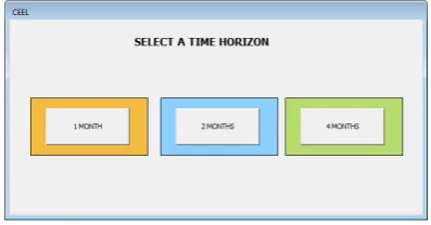
[image:22.595.199.398.136.240.2]A.4.1 Interface to select between time horizons (common to all treatments)
A.4.2 Sample choice problem - MPL
A.4.3 Sample choice problem - BDM
A.4.4 Sample choice problem - SPA
B
Predictions of Discount Rates Implied by Choices
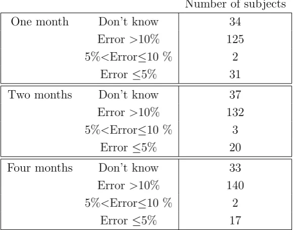
In the last phase of the experiment, we verified (in an incentived way) subjects’ percep-tions of the interest rates implied by their choices, as was indicated to subjects in the instructions. The elicitation method seems to have no effect on subject prediction errors. In Table 4, we show the distribution of prediction errors by time horizon.
Number of subjects
One month Don’t know 34
Error >10% 125
5%<Error10 % 2
Error 5% 31
Two months Don’t know 37
Error >10% 132
5%<Error10 % 3
Error 5% 20
Four months Don’t know 33
Error >10% 140
5%<Error10 % 2
[image:26.595.154.444.192.419.2]Error 5% 17
Table 4: Frequency of prediction errors, by time horizon
C
The HEXACO personality inventory
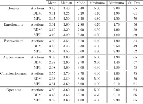
The conventional ‘Big Five’ personality traits (CANOE: Conscientiousness, Agreableness, Neuroticism, Openness, Extraversion) have been found to be unsatisfactory when used to assess personality traits in non anglophone populations (see e.g. Lee and Ahston [22]). For this reason we have instead relied on the HEXACO personality inventory, which concentrates on six personality traits: Honest, Emotionality, eXtraversion, Agreableness, Conscientiousness and Openness to experience. Each trait has five subtraits. Subjects were asked a total of 60 personality questions, with each group of 10 assessing a different trait. Given that we ’only’ have 192 subjects overall, we do not have enough data for a proper analysis using these traits as regressors. For this reason, we do not discuss personality measures in the body of the paper.
treat-ment were fairly homogeneous in terms of personality traits. We present these summary statistics both by treatment in Table 5.
Mean Median Mode Maximum Minimum St. Dev.
Honesty Auctions 3.48 3.40 3.40 5.00 2.00 .65
BDM 3.41 3.25 3.20 4.70 1.90 .61
MPL 3.47 3.50 3.30 4.80 1.50 .70
Emotionality Auctions 3.01 3.00 2.80 4.70 1.70 .56
BDM 3.19 3.20 2.90 4.50 1.90 .59
MPL 3.10 3.20 3.30 4.30 1.80 .59
Extraversion Auctions 3.50 3.55 3.70 4.40 1.90 .54
BDM 3.46 3.45 3.30 4.50 2.50 .49
MPL 3.50 3.55 3.60 4.90 2.30 .52
Agreeableness Auctions 3.08 3.00 2.80 5.00 1.90 .65
BDM 2.88 2.90 2.70 3.90 1.40 .57
MPL 2.98 3.00 3.00 4.30 1.80 .58
Conscientiousness Auctions 3.55 3.70 3.70 4.90 1.00 .75
BDM 3.63 3.80 3.80 5.00 1.90 .70
MPL 3.61 3.60 3.60 4.90 2.10 .61
Openness Auctions 3.50 3.60 4.00 5.00 2.00 .64
BDM 3.43 3.55 3.70 4.70 2.10 .66
[image:27.595.78.558.115.464.2]MPL 3.59 3.60 4.00 4.80 2.30 .65
Table 5: HEXACO personality traits - summary statistics by treatment
To evaluate whether any of the differences across treatments are statistically signifi-cant, we regress the measure of each trait above on treatment dummies. None of our tests for equality of treatment dummy coefficients reject the null hypothesis of equality in that personality trait in each treatment at the 5% significance level.
C.1
HEXACO questions
The HEXACO personality inventory questions in the English version follow below (from Lee and Ashton [22]).
DIRECTIONS
your response in the space next to the statement using the following scale: 5 = strongly agree 4 = agree 3 = neutral (neither agree nor disagree) 2 = disagree 1 = strongly disagree Please answer every statement, even if you are not completely sure of your response. Please provide the following information about yourself.
Sex (circle): Female Male
Age: years
(we also added indication of the discipline to which student participants belonged)
1. I would be quite bored by a visit to an art gallery.
2. I plan ahead and organize things, to avoid scrambling at the last minute.
3. I rarely hold a grudge, even against people who have badly wronged me.
4. I feel reasonably satisfied with myself overall.
5. I would feel afraid if I had to travel in bad weather conditions.
6. I wouldn’t use flattery to get a raise or promotion at work, even if I thought it would succeed.
7. I’m interested in learning about the history and politics of other countries.
8. I often push myself very hard when trying to achieve a goal.
9. People sometimes tell me that I am too critical of others.
10. I rarely express my opinions in group meetings.
11. I sometimes can’t help worrying about little things.
12. If I knew that I could never get caught, I would be willing to steal a million dollars.
13. I would enjoy creating a work of art, such as a novel, a song, or a painting.
14. When working on something, I don’t pay much attention to small details.
15. People sometimes tell me that I’m too stubborn.
16. I prefer jobs that involve active social interaction to those that involve working alone.
18. Having a lot of money is not especially important to me.
19. I think that paying attention to radical ideas is a waste of time.
20. I make decisions based on the feeling of the moment rather than on careful thought.
21. People think of me as someone who has a quick temper.
22. On most days, I feel cheerful and optimistic.
23. I feel like crying when I see other people crying.
24. I think that I am entitled to more respect than the average person is.
25. If I had the opportunity, I would like to attend a classical music concert.
26. When working, I sometimes have difficulties due to being disorganized.
27. My attitude toward people who have treated me badly is “forgive and forget”.
28. I feel that I am an unpopular person.
29. When it comes to physical danger, I am very fearful.
30. If I want something from someone, I will laugh at that person’s worst jokes.
31. I’ve never really enjoyed looking through an encyclopedia.
32. I do only the minimum amount of work needed to get by.
33. I tend to be lenient in judging other people.
34. In social situations, I’m usually the one who makes the first move.
35. I worry a lot less than most people do.
36. I would never accept a bribe, even if it were very large.
37. People have often told me that I have a good imagination.
38. I always try to be accurate in my work, even at the expense of time.
39. I am usually quite flexible in my opinions when people disagree with me.
41. I can handle difficult situations without needing emotional support from anyone else.
42. I would get a lot of pleasure from owning expensive luxury goods.
43. I like people who have unconventional views.
44. I make a lot of mistakes because I don’t think before I act.
45. Most people tend to get angry more quickly than I do.
46. Most people are more upbeat and dynamic than I generally am.
47. I feel strong emotions when someone close to me is going away for a long time.
48. I want people to know that I am an important person of high status.
49. I don’t think of myself as the artistic or creative type.
50. People often call me a perfectionist.
51. Even when people make a lot of mistakes, I rarely say anything negative.
52. I sometimes feel that I am a worthless person.
53. Even in an emergency I wouldn’t feel like panicking.
54. I wouldn’t pretend to like someone just to get that person to do favors for me.
55. I find it boring to discuss philosophy.
56. I prefer to do whatever comes to mind, rather than stick to a plan.
57. When people tell me that I’m wrong, my first reaction is to argue with them.
58. When I’m in a group of people, I’m often the one who speaks on behalf of the group.
59. I remain unemotional even in situations where most people get very sentimental.