Common Properties of Riemann Zeta Function, Bessel Functions and Gauss Function Concerning Their Zeros

http://www.scirp.org/journal/apm ISSN Online: 2160-0384

ISSN Print: 2160-0368

DOI: 10.4236/apm.2019.93013 Mar. 29, 2019 281 Advances in Pure Mathematics

Common Properties of Riemann Zeta Function,

Bessel Functions and Gauss Function

Concerning Their Zeros

Alfred Wünsche

Institut für Physik, Humboldt-Universität, MPG Nichtklassische Strahlung, Berlin, Germany

Abstract

The behavior of the zeros in finite Taylor series approximations of the Rie-mann Xi function (to the zeta function), of modified Bessel functions and of the Gaussian (bell) function is investigated and illustrated in the complex domain by pictures. It can be seen how the zeros in finite approximations ap-proach to the genuine zeros in the transition to higher-order approximation and in case of the Gaussian (bell) function that they go with great uniformity to infinity in the complex plane. A limiting transition from the modified Bes-sel functions to a Gaussian function is discussed and represented in pictures. In an Appendix a new building stone to a full proof of the Riemann hypothe-sis using the Second mean-value theorem is presented.

Keywords

Riemann Zeta and Xi Function, Modified Bessel Functions, Second Mean-Value Theorem or Gauss-Bonnet Theorem, Riemann Hypothesis

1. Introduction

The present paper tries to find out the common ground for the zeros of the Riemann zeta function ζ

( )

z =ζ

(

x+iy

)

and of the modified Bessel functions

( )

Iν z (or Bessel functions Jν

( )

z of imaginary argument z) for imaginary argument z and, furthermore, for the absence of zeros of the Gaussian Bell function

( )

2

exp z . For the function now called Riemann zeta function ζ

( )

z

which was known already to Euler but was extended by Riemann to the complex plane Riemann expressed the hypothesis that all nontrivial zeros of this function lie on the axis 1 i

2

z= + y that means on the axis through 1

2

x= and parallel to

How to cite this paper: Wünsche, A. (2019) Common Properties of Riemann Zeta Function, Bessel Functions and Gauss Function Concerning Their Zeros. Ad-vances in Pure Mathematics, 9, 281-316. https://doi.org/10.4236/apm.2019.93013

Received: March 1, 2019 Accepted: March 26, 2019 Published: March 29, 2019

Copyright © 2019 by author(s) and Scientific Research Publishing Inc. This work is licensed under the Creative Commons Attribution International License (CC BY 4.0).

http://creativecommons.org/licenses/by/4.0/

DOI: 10.4236/apm.2019.93013 282 Advances in Pure Mathematics the imaginary axis y (Riemann hypothesis) [1][2][3] (both with republication of Riemann’s paper) and many others, e.g. [4] [5] [6][7] [8]. Riemann never proved his hypothesis. He introduced in [1] also a Xi function ξ

( )

z which

excludes the only singularity of the function ζ

( )

z at z=1 and its trivial zeros at

z

= − −

2, 4,



and possesses more symmetry than the zeta function

( )

z

ζ . Concerning their zeros it is equivalent to the nontrivial zeros of the zeta function. In present paper we will mainly have to do only with this Xi function

( )

z

ξ _{which we displaced in a way that its zeros lie on the imaginary axis}

provided; the Riemann Hypothesis is correct and we denote as Xi function

( )

z

Ξ _{. With respect to the position of the zeros the function} Ξ

( )

z is fully

equivalent to the nontrivial zeros of the Riemann zeta function ζ

( )

z only with

displacement of the imaginary axis to these zeros.

The content of this article was not intended as a proof of the Riemann hypothesis but during the work we found a further, as it seems, essential building stone for its proof by the second mean-value approach which is represented in Appendix. The article is merely intended as an illustration to the zeros of a function with a possible representation in an integral form given in Section 2 (Equation (2.8)) with monotonically decreasing functions Ω

( )

u

satisfied by the Riemann Xi function and by the modified Bessel functions and explains why the Gauss bell function although it can be represented in such form does not possess zeros. Other kinds of interesting illustrations of the Riemann zeta function (and of other functions) by the Newton flow are given in [9] [10]. A main purpose was to understand how the zeros in the Taylor series approximations of such functions behave when we go from one order of the approximation to the next higher one. To get the possibility of a comparison with the pictures of zeros for functions without an integral representation of the mentioned form we made an analogous picture for an unorthodox entire function in Section 9.

2. Basic Equations for the Considered Functions

The Xi function Ξ

( )

z to the Riemann zeta function ζ

( )

z is defined by

( )

1

, 2

z ξ  z

Ξ ≡ _ + _

  (2.1)

where ζ

( )

z is the Riemann Xi function [1] which is related to the Riemann

zeta function ζ

( )

z by1

( ) (

₁

)

!π 2

( )

_.

2 z

z

z z z

ξ

≡ _{−  }  −

ζ

  (2.2)

The Riemann zeta function is basically defined by the following Euler product

( )

( )

(

)

1

1 2 3 4

1

1

1 _z , 2, 3, 5, 7, ,

n _n

z p p p p

p

ζ

− ∞

=

 

 

≡ − = = = =

 

 

∏

 (2.3)

1_{Riemann denotes the complex variable by s= +σ it that is ξ}( )_{s for the Xi function and ζ}( )_s

DOI: 10.4236/apm.2019.93013 283 Advances in Pure Mathematics where pn is the sequence of prime numbers beginning with p1=2. The definition of the Riemann Xi function (2.3) is equivalent to the definition by the following (Dirichlet) series for complex variable z= +x iy

( )

(

( )

)

1

1

, Re 1 ,

z n

z x z

n

ζ ∞

=

=

∑

= > _(2.4)

which is convergent for x>1 and arbitrary y and can be analytically continued to the whole complex z-plane. The function Ξ

( )

z is an entire function which

excludes the only singularity of ζ

( )

z at z=1 and its “trivial” zeros at

2, 4, 6,

z

= − − −



.

Next we consider the whole class of modified Bessel functions I_ν

( )

z of

imaginary argument which is connected with the basic class of Bessel functions

( )

J_ν z in the following slightly modified form by (µ!≡ Γ

(

µ+1

)

)

( )

( )

₍

₎

2

(

)

0

2 2 1

I J i , .

i ! ! 2

m

m

z

z z

z z m m

ν ν

ν ν _ν ν

∞

=

  ₌  _≡   _∈

    ₊  

   

∑

   (2.5)

The functions 2 I

( )

z z

ν

ν

   

  are entire functions which satisfy the differential

equation

( )

( )

2 2

2 2 2 2

2 I 0 I 0.

z z z z z z z

z z z z

ν

ν ν

ν

ν

 _{∂ ∂}   _∂ 

  _{+ −}   _{= ⇔}   _{− −}  ₌

_{ ∂} _{ ∂} _{ }  _ _∂ _ 

   

    (2.6)

In comparison to I_ν

( )

z the functions 2 I

( )

z z

ν

ν

   

  exclude the zeros or

infinities of the first ones at z=0 but the other zeros remain the same for both functions.

Finally, we consider the Gaussian functions exp 2 2 4

a z

 

 

  with parameter

2

0

a > which can be represented by the following integral representation

(continued from the imaginary axis y to the whole complex z-plane)

( )

(

)

2 2 2

2 2

0 2 2

exp d exp ch , 0 ,

4 _π

a z u

u uz a

a a

+∞

   

= − >

   

 

∫

  (2.7)

which become Gaussian bell functions for imaginary argument z=iy. Clearly,

the functions exp 2 2 4

a z

 

 

  do not possess zeros on the imaginary axis and zeros

at all.

The three mentioned types of functions written as Ξ

( )

z have in common

that they are symmetrical functions in z and that they possess a representation by an integral of the type

( )

( ) ( )

( )

(

( )

)

*

( )

( )

*

0 d ch ) , ,

z +∞ u u uz z z u u

Ξ =

_∫

Ω = Ξ − = Ξ Ω = Ω − _(2.8)

with monotonically decreasing functions Ω

( )

u for 0≤ ≤ ∞u that means

( )

( )

(

)

1 2 1 2

DOI: 10.4236/apm.2019.93013 284 Advances in Pure Mathematics The Taylor series of Ξ

( )

z can be written in the form

( )

2

(

( )

( )

)

2 0

1 1

, d

! 2

m n

m n

m

z z u u u u

n

∞ _+∞

−∞ =

Ξ =

∑

Ω Ω ≡

_∫

Ω + Ω −

( )

( )

2

(

)

2 ₀ 2 1

1

d , 0, 0,1, 2, ,

2 !

m

m u u u m m

m

+∞

+

Ω =

_∫

Ω Ω = = _{ (2.10)}

where Ω_n,

(

n=0,1, 2,

)

are defined as the moments of the symmetrical function Ω

( )

u with respect to the reference point u₀=0. A consequence of

the definitions in (2.8) and (2.10) is

( )

0 ₀ du

( )

u 0.

+∞

Ξ =

_∫

Ω ≡ Ω _(2.11)

The odd moments Ω2m+1 of the function Ω

( )

u in the definition (2.10) vanish. The function Ξ

( )

z at z=0 is equal to the zeroth moment Ω₀ of the function Ω

( )

u and is independent of the chosen reference point. In the

following the moments of the function Ω

( )

u play an important role.

That Ω

( )

u is a symmetrical function in u is, in principle, not necessary since

the integration over u in (2.8) is restricted by u≥0 but the symmetry permits to extend the integral over negative values of u using it in the form

( )

( )

( ) ( )

( ) ( )

0

1 1 1

d e d ch d sh ,

2 2 2

uz

z _−∞+∞ u u _−∞+∞ u u uz _−∞+∞ u u uz

=

Ξ =

_∫

Ω =

_∫

Ω +

_∫

Ω

 (2.12)

which for imaginary z=iy is a Fourier transformation of Ω

( )

u with the

inversion

( )

1

( )

i

d i e ,

π

uy

u _−∞+∞ y y −

Ω =

_∫

Ξ _(2.13)

if the integral exists in some sense (e.g. weak convergence). We consider this now more explicitly.

The explicit representation of the Xi function Ξ

( )

z to the Riemann Xi

function

( )

1

2

z z

ξ = Ξ_ − _

  in this form (2.8) together with (2.9) is

( )

z ₀+∞du

( ) ( )

u ch uz ,

Ξ =

_∫

Ω

( )

2 2

(

2 2

) (

2 2

)

( )

1

4 exp π e 2π e 3 exp π e ,

2

u u u

n

u

u n n n u

∞

=

 

Ω ≡ _{ } − − = Ω −

 

∑

(2.14)

with the special values

( )

₀

( )

1 1

0 d 0.4971207782, ,

2 2

u u

+∞  

Ξ = Ω ≈ Ξ ±_{ }=

 

∫

( )

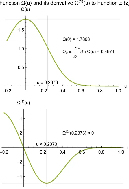
0 1.7867876019.

Ω ≈ _(2.15)

This was derived in detail in [11]. The function Ω

( )

u together with its first

derivative ( )1

( )

u

Ω is represented in Figure 1.

[image:5.595.263.486.74.402.2]

DOI: 10.4236/apm.2019.93013 285 Advances in Pure Mathematics Figure 1. Representation of Ω

( )

u and of its first derivative

( )1

_{( )}

u

Ω _{. The function} Ω

( )

u is monotonically decreasing

for u≥0 and together with its derivatives vanishes rapidly

for u→ +∞.

of Ω

( )

u is not easily to see from (2.14) and it was a genuine surprise for us to

meet such a kind of a symmetrical function (see discussion in [11]). The function exp

( )

2

u u

₋ _Ω

 

  , for example, is already not a symmetrical function for

u↔ −u.

In case of the modified Bessel functions of imaginary argument the following basic integral representations are known which for the functions proportional to

( )

2 I z z

ν

ν

   

  may be written as follows (taking into account

1 1 1 π

! !

2 2 2 2

  ₌ ₋  ₌

   

    )

( )

( )

(

)

( )

( )

( )

1

1 ₂

2 0

0 d 1 ch

1 1 2 1

0 ! ! I , ,

2 2 2

z u u uz

z z

ν

ν ν

ν

ν ν ν ν

−

Ξ ≡ Ω −

       

= Ω _{  } − _{   } > − _

       

∫

(2.16)

DOI: 10.4236/apm.2019.93013 286 Advances in Pure Mathematics

( )

( )

1 1

1 1

! !

1

2 2

0 e F ; 2 1; 2 .

! 2 z z z ν ν ν ν ν ν    ₋      _{ }    

Ξ = Ω _ + + ± _

 

 _(2.17)

The Taylor series expansion is

( )

( )

₍

₎

2

1

1 1

! !

!

2 2

0 1 .

! ! ! 2

m m z z m m ν ν

ν

ν

ν

ν

∞ =    ₋     _{    }    

Ξ = Ω _ + _{  }

+  

 



∑

 (2.18)

The functions Ξ_ν

( )

z possess the principal form

( )

₀

( ) ( )

1

d ch , ,

2

z u u uz

ν ν ν

+∞  

Ξ = Ω _ > − _

 

∫

(2.19)

with the following explicit expressions for Ων

( )

u

( )

( )

(

2

)

1₂

(

2

)

( )

0 1 1 ,

u u ν u u

ν ν θ ν

−

Ω = Ω − − = Ω − (2.20) where θ

( )

x is Heaviside’s step function defined by

( )

1,

(

₍

0 ,

)

₎

0, 0 .

x x

x θ ≡  >_<

 (2.21)

It restricts the upper limit of integration in (2.19) according to the choice in (2.20) to u=1. The functions Ω_ν

( )

u are equivalent to functions of u2 only

and are in this sense symmetrical functions of u and for real 2

1

u < we have to

choose the real value of

(

₁−_u2

)

ν−12 in case of non-integer 1

2 ν − _.

The first six cases of the function Ξ_ν

( )

z with integer or semi-integer index

ν are

( )

( )

( )

( )

( ) ( )

( )

( ) ( )

( )

( )

(

( )

( )

)

( )

( )

( )

( )

( )

(

(

)

( )

( )

)

0

0 0 1 1

2 2

1

1 1 3 3 3

2 2

2 2

2 2 2 5 5 5

2 2

πI sh

0 , 0 ,

2

2 ch sh

πI

0 , 0 ,

2

8 3 sh 3 ch

3πI

0 , 0 .

2

z z

z z

z

z z z

z

z z

z z

z z z z

z

z z

z z

Ξ = Ω Ξ = Ω

−

Ξ = Ω Ξ = Ω

+ −

Ξ = Ω Ξ = Ω

(2.22)

The function 1

( )

2

z

−

Ξ does not exist since the corresponding integral in (2.16) is divergent or 1 !

2 ν

 ₋ 

 

  is not finite for 1 2 ν = − _but

( )

_{( )}

1 2 1 2 ch lim 1 2 ! 2 z z ν ν − →− Ξ =  ₋     

exists. Furthermore, we have introduced in (2.16)

amplitudes Ω_ν

( )

0 and we will soon see that it is favorable to choose them for our purpose as constant for the whole class of functions Ξν

( )

z . We illustrate

the functions Ω_ν

( )

u and the corresponding functions Ξ_ν

( )

z with a certain

important modification in next Section 3.

DOI: 10.4236/apm.2019.93013 287 Advances in Pure Mathematics real axis x and, correspondingly, I_ν

( )

z only on the imaginary axis y. For this

there exists a direct proof using their differential equations and which is similar to the derivation of duality and orthogonality relations (e.g. [12][13]).

The considered Omega functions Ω

( )

u for the Riemann Xi function and

( )

u

ν

Ω for the modified Bessel functions and also for the Gaussian bell function have in common that they are monotonically decreasing functions for u≥0 up to Ω +∞ =

( )

0.

3. Modified Bessel Functions with Stretched Argument

of the Kernel Function and Limiting Transition to

Gaussian Bell Function

We now calculate the even moments Ων,2m of the functions Ων

( )

u in (2.20) which lead to well-known integrals

( )

( )

( )

( )

(

)

( ) ( ) ( )

( )

₍

₎

1 1

2 2 2 2

,2 _{0 0}

2

0 1

d d 1

2 ! 2 !

1 1 1 1

! ! ! !

1 π

2 2 2 2

0 0 , ! ,

2 2 ! ! ! !2 2 2

m m

m

m

u u u u u u

m m

m

m m m m

ν ν ν ν ν ν

ν

ν

ν

ν

− +∞ Ω

Ω ≡ Ω = −

 ₋   ₋     ₋ 

        _{  }

       

= Ω ₊ = Ω _{ } = _

+ _  _

∫

∫

(3.1)

and in the special case m=0 of zeroth moments

( )

,0 1 1 ! ! 2 2 0 . ! ν ν ν ν    ₋         

Ω = Ω _(3.2)

These are the areas under the curves Ω_ν

( )

u on the positive u-axes. The

following considerations show that it is favorable to make Ων,0 equal

independently on parameter ν _{and to keep} Ω_ν

( )

0 constant and we choose

( )

0 1. ν

Ω = _(3.3)

To keep in addition also Ων,0 constant we have now the only possibility to

introduce a stretch factor to the variable u and we make the transformation (now already with choice (3.3))

( )

( )

1

2 2 2

2 2

,0

,0 ,0

1 u 1 u u ,

u u

u

u u

ν

ν ν ν

ν

ν ν

θ

−

     

Ω → Ω =_ − _{ } − _= Ω _ _  

    (3.4)

with the definition of uν,0

1 ,0 2

,0 1 1

,0 ,0 ,0 2 2 ! , 1, 1 1 ! ! 2 2 u

u_ν u u

ν ν ν ≡ = = Ω    ₋          (3.5)

from which follows for the zeroth moments of Ω_ν

( )

u

( )

,0

1 2 2

,0 0 0 2

,0

du u u du 1 u 1.

u ν ν ν ν ν − +∞  

Ω ≡ Ω = _ − _ =

 

∫

∫

(3.6)

[image:8.595.98.538.84.383.2]

DOI: 10.4236/apm.2019.93013 288 Advances in Pure Mathematics Figure 2. Functions Ω_ν

( )

u with stretched variable

,0

u u

uν

→ _{in comparison to functions} Ω_ν

( )

u . G rid lines are set

at the values uν,0 where the finite functions Ων

( )

u end. In the chosen scale the curve Ων

( )

u for

9 2

ν = is visibly

already hardly to distinguish from a Gaussian bell function exp π 2 4

u

 

−

 

  and, therefore, is not drawn here.

values of ν _{up to} 9

2

ν = _.

The corresponding transformation of the functions Ξ_ν

( )

z using (2.16) and

(3.3) are

( )

( )

(

)

(

)

,0

1

2 2

,0 0 2 ,0

,0 ,0 ,0

,0 ,0 ,0

,0

d

1 ch

2

! I .

u u u u

z z u u z

u u u

u u z u z u z

ν

ν

ν ν ν ν

ν ν ν

ν

ν ν ν ν ν

ν

ν

−

   

Ξ → Ξ = _ − _ _ _

 

 

 

= Ξ = _ _

 

∫

(3.7)

Their Taylor series are

( )

₍

₎

(

)

( )

2 ,0

0

2

1 !

! ! 2

! !

1 ,

1 1

! ! 2

! !

2 2

m

m

m

m

u z

z

m m

z

z

m m

ν ν

νν

ν ν

ν ν

ν _ν

∞

=

∞

=

 

Ξ = _{ }

+ _{ }

 

 

 

= + = Ξ −

+    ₋       _{   } 

 

∑

∑

DOI: 10.4236/apm.2019.93013 289 Advances in Pure Mathematics or with substitution z=iy (see also (2.5))

( )

(

)

( )

(

)

,0 ,0 2 1 2

i ! J

1 ! !

1 .

1 1

! ! 2

! !

2 2

m

m

m

y u y

u y

y

m m

ν

ν ν ν

ν ν ν ν ν _ν ∞ =  

Ξ = _ _

      − _{ } = + +    ₋       _{   }   

∑

 (3.9)

The first three functions Ξ_ν

( )

z with integer and with semi-integer ν are

explicitly

( )

( )

( )

( )

( )

( )

( )

(

)

0 0 1

2

1 1 3 3

2

2 2

2 2 2 5 5

2 sh 2

I , ,

π

3 3

4 3 ch 2sh

2 2

π 4

I , ,

2 π 9

15 15

512 64 75 sh 120 ch

8 8

9π 16

I , .

3π 32 16875 z z z z z z z z z z z z z z z z z z z z z z  

Ξ = _{ } Ξ =

 

  ₋  

   

 

      

Ξ = _{ } Ξ =

 

 ₊  ₋  

   

 

      

Ξ = _{ } Ξ =

 

(3.10) The functions Ξ_ν

( )

z on the imaginary axes z=iy for integer and

semi-integer index ν _{up to} 9

2

ν = _{are illustrated in Figure 3.}

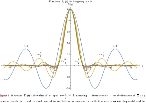
Figure 2 and Figure 3 admit the conjecture that Ων

( )

u and Ξν

( )

iy for real variable y become Gaussian bell functions in the limit ν → ∞_{. For}

9 2

ν = _{in Figure 2 the function} Ω_ν

_{( )}

u is in visible way already hardly to

distinguish from the Gaussian bell function (below we see to exp π 2 4 u   −    ).

That the mentioned approach for ν → ∞ _{to a Gaussian bell function is really}

true we establish exactly and determine these limits.

We now show that the new functions Ξ_ν

( )

z in (3.7) for ν → ∞ go to a

Gaussian function that becomes a Gaussian bell function for imaginary z=iy.

As auxiliary formulae for !

1 ! 2 ν ν  ₋     

in case of ν 1 follows

( )

(

)

1 2 1 !

! 2 1 1 ! 1

,

1 1 ! 4 4 1 4

! !

2 _{ϕ ν} 2

ϕ ν

ν

ν _{ν ν ν} ν _{ν ν}

ν ν ν   ≡ _ − _   ≡  ₋     _{ = ≈ + − ⇒ ≈ + →} −  ₋   ₋           

! 2 1 2 1 π

, ! ,

1 1 π 4 π 2 2

! !

2 2

ν _{ν ν}

[image:9.595.151.542.76.749.2]

[image:10.595.58.541.72.415.2]

DOI: 10.4236/apm.2019.93013 290 Advances in Pure Mathematics Figure 3. Functions Ξν

( )

iy for values of ν up to

9 2

ν = . W ith increasing ν from a certain ν on the first zeros of Ξ_ν

( )

z

increase (see also text) and the amplitudes of the oscillations decrease and in the limiting case ν → +∞ they vanish and the resulting Gaussian function

2 exp

π

y

  −  

  (on the imaginary y-axis z=iy) does not possess zeros. This Gaussian curve is not well to distinguish in the bulk of the other curves and is not drawn here.

and analogously for ν1

(

!

) (

! 1

)(

12

) (

)

1 12 .

1 1 1

m

m m

m m

ν _ν

ν ν ν ν _ν

ν ν ν

−

= = ≈

+ + + +  ₊  ₊   ₊ 

    

    

 _ (3.12)

Applying these approximations we find from (3.8)

(

)

2

0

2 ₂

0 0

2

! !

lim ( ) _lim

1 1

! ! 2

! !

2 2

2 1

lim

! π2 ! π

exp .

π

m

m

m m

m

m m

z z

m m

z z

m m

z

ν

ν ν

ν

ν ν

ν _ν

ν _ν

∞

→∞ _{→∞ =}

−

∞ ∞

→∞ = =

 

 

 

Ξ =

+    ₋  

   

_{   } 

 

 

 

= _{ } = _{ }

   

 

= _{ }

 

∑

∑

∑

(3.13)

This means that in the limiting transition ν → ∞ _{the functions} Ξ_ν

( )

z in

DOI: 10.4236/apm.2019.93013 291 Advances in Pure Mathematics 2

1 1

2 ! !

!

2 2

lim ! I exp ,

1 1

! 2 π

! ! 2 2 z z z ν ν ν ν ν ν ν _ν →∞     ₋          _{   }    _{ }     =        ₋   _{ }       _{   }      (3.14)

or by substitution z=iy with, in general, complex variable y

2

1 1

2 ! !

!

2 2

lim ! J exp ,

1 1

! 2 π

! ! 2 2 y y y ν ν ν ν ν ν ν _ν →∞     ₋          _{   }    _{ }     = _− _      ₋   _{ }       _{   }      (3.15)

where we use the identity 2 1 ! 1 ! π

2 2

  _{= −}  ₌

   

    . From the corresponding

limiting transition lim_ν→∞Ω_ν

( )

u using the definition in (3.4) we find

1

2 ₂ 2

2

2 2

1 1 1 1

! ! ! !

π

2 2 2 2

lim 1 1 exp .

! ! 4

u u u ν ν ν ν θ ν ν − →∞  _{    }   _{    }   _{  } − _{ }   _{  } − _{ }             _{− }   _{− } _{= − }  _{ }   _{ }  _{ }  _{ }   _{ }   _{ }   _{ }      (3.16)

We may check the transition from

( )

exp π 2 4

u

u  

Ω = _− _

  to

( )

2 exp

π

z

z  

Ξ = _{ }

 

via (2.8) using the auxiliary formula (2.7) with 2 4

π

a = .

Furthermore, we find using the approximation (3.11) that the factor between

1 ,0 2

u and uν,0 in (3.5) approaches for ν 1 according to

(

)

,0

1 ,0 2

! 2 1

, 1 ,

1 1 π 4

! !

2 2

u u

ν ν _{ν ν}

ν

= ≈ +

   ₋         

 (3.17)

with a high precision and monotonically increasing without a finite limit.

We now show that for high increasing ν 1 the first positive roots of

( )

iy

νν

Ξ and thus also the higher roots increase. For Ξ_ν

( )

iy this is clear since

it is proportional to J_ν

( )

y and it is well known that their roots

(

)

,s, 1, 2,

y_ν s=  are situated approximately at

, 1 π .

2 4

s

y_ν =_s+ −ν _ −

   (3.18)

However in Ξ_ν

( )

iy the argument in the Bessel functions is stretched by the

factor uν,0 and therefore on the imaginary axis we have the functions

(

,0

)

Jν uν y that diminishes the values for the roots (3.18) by the factor uν,01

− _and

with the approximation (3.17) the zeros of Ξ_ν

( )

iy are now situated approximately

at 3 2 , ,0 1 π 2 4 . 4 1 s s y u ν ν

ν

ν

 _{+ −}      ≈

DOI: 10.4236/apm.2019.93013 292 Advances in Pure Mathematics Thus the first roots

(

s=1

)

of Ξ_ν

( )

iy go with ν → ∞ proportional to ν _{also to infinity. This explains more in detail why the first zeros}

₍

s=1

₎

of the curves for Ξ_ν

( )

iy in Figure 3 go to the limiting case

2

exp π

y

₋ 

 

  for

ν → ∞_.

We remind that the starting point for the derivation of the approximations was making equal the zeroth moments Ων,0 by stretching the argument of the

functions Ων

( )

u to new functions Ων

( )

u leaving constant the amplitudes

( )

0 ν

Ω _{. The zeros of} Ω_ν

( )

u for ν → ∞ move in this process also to infinity

but “very slowly”. This is a good illustration why the Gaussian function

2 exp

π

z

   

  which on the imaginary axis y becomes a Gaussian bell function

2 exp

π

y

  −  

  does not possess zeros at all although its Omega function

( )

exp π 2 4

u

u  

Ω = − 

  is monotonically decreasing. The first zero and in this way

all other zeros are moved by the limiting transition to infinity although very slowly. The same is the case with the discontinuities of derivatives in the functions Ω_ν

( )

u .

4. Graphical Representations to Zeros of the Xi Function

to Riemann Zeta Function in Approximations by

Truncated Taylor Series

In this Section we consider the Taylor series expansions of the Xi function

( )

z

Ξ to the Riemann Xi function ξ

( )

s in powers of z defined in (2.14)

according to

( )

( ) ( )

( )

_{( )}

( )

0

2

2 2

2

0 0

d ch

0 ,

2 !

m

m m

m

m m

z u u uz

z z

m

+∞

∞ ∞

= =

Ξ = Ω

Ξ

= Ω =

∫

∑

∑

( )

( )

( )

_{( )}

( )

2 2

2 ₀

0 1

d .

2 ! 2 !

m m

m u u u

m m

+∞ Ξ

Ω ≡

_∫

Ω = (4.1)

The coefficients in this Taylor series are the even moments Ω2m of the

function Ω

( )

u as defined.

We truncate the Taylor series of Ξ

( )

z at upper summation numbers m=M

( )

2

2 2

0

, M

m

M m

m

z z

=

Ξ =

∑

Ω _(4.2)

and calculate all zeros of these approximations up to a certain maximal M and make graphical representations of their zeros. As mentioned the coefficients of the series are determined by the even moments Ω2m of the function Ω

( )

u

DOI: 10.4236/apm.2019.93013 293 Advances in Pure Mathematics symmetrical functions according to (2.8) and (2.10). In the following Sections we discuss the same also for modified Bessel functions I_ν

( )

z (in particular for

1 2

ν = _{) and for the limiting transition to a Gaussian function and compare this}

with the zeros for the Xi function (2.14) to the Riemann zeta function. In each approximation Ξ2M

( )

z of the Taylor series we find 2M complex zeros. It was very interesting to see which difference appears between the zeros on the imaginary axis and the bulk of the other zeros with increasing number M. This is best seen in graphical representations of the zeros.

For the function Ω

( )

u related to the Riemann hypothesis which is explicitly

given in (2.14) we calculated this series numerically up to 2M =100 with sufficiently high precision and obtained the following numerical coefficients (we write here explicitly down only a few of the obtained coefficients)2

( )

2 2

4 4 7 6

9 8 68 48

72 50 75 52

0.497120778188314 1.14859721575727 10

1.23452018070318 10 8.32355481385527 10

3.99222655134413 10 1.05272334981972 10

4.68273888631736 10 1.97190495510121 10

z z

z z

z z

z z

−

− −

− −

− −

Ξ = + ×

+ × + ×

+ × + + ×

+ × + ×



79 54 82 56

85 58 89 60

92 62 158 98

162 100

7.87602897895070 10 2.98910175366638 10

1.07971892491186 10 3.71787541158066 10

1.22215971011433 10 3.09393689867254 10

5.11093592293365 10

z z

z z

z z

z

− −

− −

− −

−

+ × + ×

+ × + ×

+ × + + ×

+ × +

 

(4.3) It is interesting to mention that the coefficients

( )

2m !Ω2m,

(

m=1, 2,

)

possess an absolute minimum for m=21 with

( )

( )

7

42

42 !Ω 0 =1.1837577 10× − and, apparently, are (“slowly”) monotonically increasing for m>21=42.

The first term in (4.3) can also be written (see [11])

( )

(

)

(

)

2 2 1

1

2 4 1

1

0.497120778188313661

1 d

0 exp π

2 2

1

d exp π

2

0.5 0.002879221811686339, n

n

t

n t t

s n s

∞ +∞

= ∞

+∞

=

≈ Ξ = − −

= − −

≈ −

∑

∫

∑

∫

(4.4)

corresponding to the splitting of terms in the representation (2.14) of Ξ

( )

z

after the substitution 2

eu = =t s .

In the truncation of the series in powers of z with the highest term proportional to 2M

z we found by numerical solution of the corresponding

algebraic equations of degree 2M the 2M complex solutions from which the

2_{We made the calculations two times with “Mathematica 3” (up to 2M = 80 and 18 digits) and with}

[image:14.595.207.538.132.490.2]

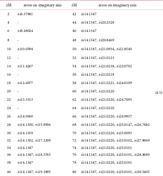
DOI: 10.4236/apm.2019.93013 294 Advances in Pure Mathematics following pairs of zeros lie on the imaginary axis z=iy3:

Table 1. Zeros zk= ±iyk on the imaginary axis for the first 2M approximations up to 2M = 80.

2M zeros on imaginary axis 2M zeros on imaginary axis 2 ±i6.57881 42 ±i14.1347

(4.5) 4 - 44 ±i14.1347, ±i20.2528

6 ±i8.48024 46 ±i14.1347

8 - 48 ±i14.1347, ±i20.8469

10 ±i10.0594 50 ±i14.1347, ±i21.0934, ±i21.8540 12 - 52 ±i14.1347, ±i21.0123

14 ±i11.4267 54 ±i14.1347, ±i21.0238, ±i23.0702 16 - 56 ±i14.1347, ±i21.0218

18 ±i12.6077 58 ±i14.1347, ±i21.0221, ±i24.0109 20 - 60 ±i14.1347, ±i21.0220

22 ±i13.5513 62 ±i14.1347, ±i21.0220, ±i24.7095 24 - 64 ±i14.1347, ±i21.0220

26 ±i14.0560 66 ±i14.1347, ±i21.0220, ±i24.9857

28 ±i14.1530, ±i15.8936 68 ±i14.1347, ±i21.0220, ±i25.0147, ±i26.7482 30 ±i14.1319 70 ±i14.1347, ±i21.0220, ±i25.0093

32 ±i14.1352, ±i17.2309 72 ±i14.1347, ±i21.0220, ±i25.0102, ±i27.8069 34 ±i14.1347 74 ±i14.1347, ±i21.0220, ±i25.0101

36 ±i14.1347, ±i18.3765 76 ±i14.1347, ±i21.0220, ±i25.0101, ±i28.8689 38 ±i14.1347 78 ±i14.1347, ±i21.0220, ±i25.0101

40 ±i14.1347, ±i19.3895 80 ±i14.1347, ±i21.0220, ±i25.0101, ±i30.5405

In the following we give graphical illustrations of all zeros of the Taylor approximations in the complex z-plane where all zeros up to a certain order 2M

are taken into account and where one may see how the zeros change from an order to a higher order.

We explain first how the following figures are made. We take a certain order 2M of the Xi function Ξ

( )

z given by the truncated Taylor series (4.2) and

determine numerically all of its zeros and represents them by points in the complex

(

z= +x iy

)

-plane where we choose the same scale on the x- and y-axis. Two variants are made, first the representation by isolated points and

3_{From about 2M=50 on the values given in the third and fourth column on the right-hand side}

DOI: 10.4236/apm.2019.93013 295 Advances in Pure Mathematics second the representation by connected neighbored points. The obtained partial pictures are a little different for odd and even M that is represented in Figure 4

for M =29 and M =30.

Then we calculate and represent all zeros of the Taylor approximations of

( )

2M z

Ξ _{(i.e. of} Ξ_2M

( )

z =0) up to a certain maximal M and represent the zeros in described way by isolated points and by connected neighbored points in each of the approximations up to the maximal M. This is made in Figure 5 and

Figure 6 for maximal 2M =60. These approximations capture already approximations of the first two nontrivial zeros of the Riemann zeta function on the positive y-axis at y1≈14.135 and at y2 ≈21.022 seen in Figure 5 by some accumulation of points at these values. Figure 6 shows the same picture with all neighbored points in each approximation joined as described. Since not all details are well recognizable in Figure 6 the same is made in Figure 7 but

Figure 4. Zeros of

( )

z 0 du

( ) ( )

u ch uz

+∞

Ξ =

_∫

Ω _for Ω

_{( )}

u according to (2.14) (i.e. for Riemann hypothesis) in approximation of

the Taylor series 2 2 0

M _m

m m=Ω z

∑

with 2M=58 and 2M =60. The obtained 58, respectively, 60 zeros are shown in the complex

plane as points without mutual distortion of the axis lengths. In the pictures to the right-hand sides we have joined neighbored numbers. On the imaginary axes where it is not clear which zeros are neighbored to zeros off the axis we went in clockwise sense on the positive part first to the highest zero and then to the next lower zeros and so on and then from the lowest zero on the imaginary axis clockwise to the next complex zero. This shows also the way we went in the next picture where the details on the imaginary axis are not so clearly visible. The two zeros at y1≈ ±14.135 and at y2≈ ±21.022 on the positive and negative

[image:15.595.61.538.276.603.2]

[image:16.595.143.536.74.309.2]

DOI: 10.4236/apm.2019.93013 296 Advances in Pure Mathematics Figure 5. Zeros of Xi function Ξ

( )

z to Riemann zeta function in the first 30 approximation

( )

2

2 0 2

M _m

M z m= mz

Ξ =

∑

Ω _{of its Taylor series with} 2M =2, 4,,60. The neighbored zeros are not joined in

each approximation. We see already the beginning accumulation of points at the first two genuine zeros of the Riemann zeta function at y1≈ ±14.135 and y2≈ ±21.022.

Figure 6. Zeros of Xi function Ξ

( )

z to Riemann zeta function in the first 30 approximation

( )

2

2 0 2

M m

M z m= mz

Ξ =

∑

Ω of its Taylor series with 2M =2, 4,,60. The neighbored zeros are joined in each

[image:16.595.145.539.397.647.2]

DOI: 10.4236/apm.2019.93013 297 Advances in Pure Mathematics Figure 7. Zeros of Xi function Ξ

( )

z to Riemann zeta function in the first 20 approximation

( )

2

2 0 2

M _m

M z m= mz

Ξ =

∑

Ω _{of its Taylor series with} 2M =2, 4,, 40. The neighbored zeros are joined in each

approximation separately. We see that the zeros of the main bulk in the approximations go slowly but with great regularity (though not proved) to infinity for M → ∞ and vanish in this way as zeros of the whole

function. Only the first zero at y1= ±14.135 as genuine zeros of the Riemann zeta function are seen here

as decoupled and stabilized.

only for the first 40 Taylor approximations where this is clearer to see. These pictures show that the zeros on the imaginary axis stabilize from order to higher orders at the genuine zeros of the Riemann zeta function on the y-axis and separate themselves from the main bulk of zeros in a considered order which do not lie on the imaginary axis. That this remains in this way for M→ ∞ is,

clearly, only a conjecture but in Section 8 we try to understand this by some analytic approximations.

In Figure 7 for the case 2M =40 we see only one accumulation point of the zeros on the positive and negative y-axis corresponding to the two zeros

1 14.135

y ≈ ± . The four higher zeros on the positive y-axis (correspondingly

negative y-axis) belong already to not yet stabilized approximations to the second zeros at y2≈ ±21.022.

It is interesting to compare the functions Ω

( )

u and Ξ

( )

z to the Riemann

zeta function with a corresponding Gaussian functions ΩG

( )

u and ΞG

( )

z

where the two parameters of the Gaussian function ΩG

( )

u which are the

amplitude and the stretching of the parameter u are chosen in the way that the first two terms of the Taylor series approximation are equal. For the function

( )

u

[image:17.595.142.538.74.354.2]

DOI: 10.4236/apm.2019.93013 298 Advances in Pure Mathematics

( )

( )

( )2

( )

2 ( )4

( )

4

2 4

0 0

0

2! 4!

1.78678760 16.7305008 67.6802 ,

u u u

u u

Ω Ω

Ω = Ω + + +

≈ − + −





(4.6)

this means for the Gaussian function ΩG

( )

u

( )

( )

( )

_{( )}

( )

( )

( )

( )

( )

_{( )}

(

)

( )

(

)

2 2 G

2 2 2

2 4

2

2

2 4

0 0 exp

2 0

0 0

0

2 2!2 0

1.78678760 exp 9.363452465

1.78678760 16.7305008 78.3276 .

u u

u u

u

u u

Ω 

Ω = Ω _ _

Ω

 

Ω Ω

= Ω + + +

Ω

≈ ⋅ −

≈ − + −





(4.7)

One may check that generally

( )

( )

G u u 0.

Ω ≥ Ω > _(4.8)

For the moments of these functions result the inequalities (

m

=

0,1, 2,



)

( )

( )

2

( )

( )

2

G,2 ₀ G ₀ 2

1 1

d d 0,

2 ! 2 !

m m

m u u u u u u m

m m

∞ ∞

Ω ≡

_∫

Ω >

_∫

Ω = Ω >

( )2

_{( ) ( )}

_{( )}

( )2

_{( )}

G 0 2 ! G,2 2 ! 2 0 .

m m

m m

m m

Ξ ≡ Ω > Ω ≡ Ξ (4.9)

The resulting function ΞG

( )

z is a Gaussian function of the complex variable

i

z= +x y

( )

( )

_{( )}

( )

( )

( )

( )

_{( )}

(

)

2

G 2 2

2

π 0 0

0 exp

2 0 2 0

0.517487503 exp 0.0266995535 .

z z

z

 

Ω Ω

Ξ = Ω −  − 

 

Ω _ Ω _

≈ ⋅

(4.10)

It possesses another amplitude in comparison to Ξ

( )

z (i.e. to 0.497120778).

Clearly, as a Gaussian function it does not possess zeros on the y-axis and zeros at all. The Ω

( )

u function to the Riemann Xi function and the considered

modified Bessel functions possess the common property that they vanish in infinity more rapidly (or are even finite) than the Omega function to a Gauss function. In principle, this does not exclude Omega functions which vanish less rapidly. For example, a function

( )

e ,u

(

0, Re

( )

0

)

u α u α

Ω = ≥ > provides

( )

z 2 2

z

α

α

Ξ =

− without zeros of Ξ

( )

z at all in finite regions of the complex

plane but with poles that regarding the zeros is the same as for a Gauss function (see Section 8 where this is explained by motion to infinity from finite approximations). However, by comparison with Gauss functions we may get inequalities for the moments of the considered Omega functions.

5. Zeros of the Taylor Series Approximations of the

Function

( )

z

z

sh

DOI: 10.4236/apm.2019.93013 299 Advances in Pure Mathematics (3.7) to the Omega functions Ω_ν

( )

u in (3.4). From this class of functions

which in the limit ν → ∞ _{go to a Gaussian function we choose the function}

( )

sh z z

( )

( )

( )

1 1

2 2

sh ,

z

z z

z

Ξ = Ξ = _(5.1)

and give graphical representations of the zeros for its Taylor series approximations

( )

( )

₍

2

₎

2

1 1

,2 ,2

0 0

2 2

1 ! 2

. 1

2 1 ! 2

! !

2

m m

M M

M M

m m

z z

z z

m

m m

= =

 

  _{ }

 

Ξ = Ξ = = _{ }

+  ₊   

 

 

∑

∑

(5.2)

They are represented in Figure 8 and in Figure 9 up to the approximation for 2M =60 with the difference that in the first all zeros are presented together and in the second we have joined the neighbored zeros in each approximations. The genuine zeros of sh

( )

z

[image:19.595.58.539.235.692.2]

z lie at z0 =nπ according to

Figure 8. Zeros of the function

( )

( )

0

₍

2

₎

sh

2 1 ! m m

z z

z

z m

∞ =

Ξ = =

+

∑

in the first 30 approximations 2

( )

0

₍

2

₎

2 1 ! m M

M m

z z

m =

Ξ =

+

∑

of its Taylor series with 2M =2, 4,,60. The neighbors within an approximations are not joined and it is not fully easy to see which

[image:20.595.63.540.66.425.2]

DOI: 10.4236/apm.2019.93013 300 Advances in Pure Mathematics Figure 9. Zeros of the function

( )

( )

0

₍

2

₎

sh

2 1 ! m m

z z

z

z m

∞ =

Ξ = =

+

∑

in the first 30 approximations 2

( )

0

₍

₂ 2 _{1 !}

₎

m M

M m

z z

m =

Ξ =

+

∑

of its Taylor series with 2M =2, 4,,60. The neighbors within each approximations are here joined. Since in each approximation a

point on the positive imaginary goes approximately to the first zeros at y1= ±π the connections on the imaginary axis are not

easily recognizable.

(

)

( )

0

0

0 sh

π, 1, 2, z 0.

z in n

z

= = ± ±  ⇒ = (5.3) We may expect that for other low values of index ν ≥0 in the functions

( )

z

ν

Ξ _{we get similar illustrations with small topological distortions of the}

pictures for 1

( )

( )

2

sh z z

z

Ξ = _.

The function sh

( )

z

z possesses a peculiar importance since for monotonically

decreasing functions Ω

( )

u (for 0≤ < +∞u with Ω +∞ =

( )

0) we may apply the second mean-value theorem (Gauss-Bonnet theorem; see, e.g. Courant [14]

(chap. IV), Widder [15]) to bring the integral (2.14) to the form

( )

( ) ( )

( )

(

0

( )

)

0

sh

d ch 0 w z z .

z u u uz

z

+∞

Ξ =

_∫

Ω = Ω _(5.4)

Herein, w0

( )

z is a mean value function from which we may assume that it is

DOI: 10.4236/apm.2019.93013 301 Advances in Pure Mathematics analytically on z. In next Section we consider shortly the problem of zeros of the function Ξ

( )

z of the form (5.4).

6. General Conditions for Zeros of Functions

(

w

( )

z z

)

z

0

sh

The problem of zeros of functions Ξ

( )

z of the form (5.4) leads essentially to

the problem of zeros of sh

(

w0

( )

z z

)

with exclusion of the zero at z=0. If we separate the real and imaginary part of w0

( )

z according to

( )

( )

( )

0 0 , i 0 , , i ,

w z =u x y + v x y z= +x y (6.1)

and if we then separate the real and imaginary part of sh

(

w0

( )

z z

)

the function (5.4) can be written in the form (the separation of real and imaginary part in the first factor is uninteresting since a zero at z=0 is excluded)

(

)

( )

(

(

)

(

)

(

(

)

(

)

)

)

( )

_{

₍

₍

₎

₍

₎

₎

₍

₍

₎

₍

₎

₎

(

)

(

)

(

)

(

(

)

(

)

)

}

0 0 0 0

0 0 0 0

0 0 0 0

0

i sh , , i , ,

i

0

sh , , cos , ,

i

ich , , sin , , .

x y u x y x v x y y u x y y v x y x

x y

u x y x v x y y u x y y v x y x

x y

u x y x v x y y u x y y v x y x

Ω

Ξ + = − + +

+ Ω

= − +

+

+ − +

(6.2)

From both forms of the right-hand side in (6.2) we find that for zeros of

(

x iy

)

Ξ + _{the following two conditions [11]}

(

)

(

)

0 , 0 , π, 1, 2, ,

u x y y+v x y x=n n= ± ± 

(

)

(

)

0 , 0 , 0,

u x y x−v x y y= (6.3)

have to be satisfied at the same time and this is necessary and sufficient.

We now consider the special case of Ξ

( )

z on the imaginary axis y and find

from (6.2)

( )

( )

(

(

(

)

(

)

)

)

( )

(

0

( )

)

0 0

sin 0

iy sin u 0,y iv 0,y y 0 w y y .

y y

Ω

Ξ = + = Ω (6.4)

Since due to symmetries (2.8) the function Ξ

( )

iy has to be a real-valued

function that for y≠0 in (6.4) is only possible if v0

(

0,y

)

vanishes we find

on the imaginary axis

( )

( )

( )

(

( )

)

( ) ( )

0 0 ₀

0

0, 0 i sin 0, d cos .

v y y u y y u u uy y

+∞

Ω

= ⇒ Ξ = =

_∫

Ω _(6.5)

This follows also immediately by application of the second mean-value theorem to the integral for Ξ

( )

iy where the mean value can only take on real

values here in dependence on y as parameter. Thus for zeros on the imaginary axis

(

x=0

)

the two conditions (6.3) reduce to only one condition

( )

0 0, π, 1, 2, .

u y y=n n= ± ±  (6.6)

DOI: 10.4236/apm.2019.93013 302 Advances in Pure Mathematics axis analytically or, at least, numerically but for many problems including the considered one it is not necessary to know these zeros explicitly.

We return to the general case of general values x on the real axis with the conditions (6.3) for zeros. From (2.8) follows that Ξ

( )

z should be an analytic

function for all z for which the integral exists that means to satisfy the Cauchy- Riemann equations. For a general analytic function

( )

(

i

)

(

,

)

i

(

,

)

w z =w x+ y =u x y + v x y one can derive by integration of the

Cauchy-Riemann equations the following relations in case of v

(

0,y

)

=0 [11]

( )

, cos

( )

0, ,

( )

, sin

( )

0, .

u x y x u y v x y x u y

y y

 ∂   ∂ 

= _{ } = − _{ }

∂ ∂

    (6.7)

Now come into play the following operator identities (operator identities are such identities which can be applied to arbitrary functions to provide function identities) [11]

cos x y ycos x xsin x ,

y y y

 ∂  ₌  ∂ ₋  ∂ 

 _∂   _∂   _∂ 

     

sin x y xcos x ysin x .

y y y

 ∂  ₌  ∂ ₊  ∂ 

 _∂   _∂   _∂ 

      (6.8)

More general identities of such kind can be derived by representing the Cosine and Sine functions by Exponential functions and using that exp ix

y

_± ∂ 

 _∂ 

 

applied to analytic functions f y

( )

displace the argument of these functions to

(

i

)

f y± x that is discussed in [11]. Using (6.7) and (6.8) we may write the

conditions for zeros (6.3) in the following way

( )

(

)

0 0

π cos sin 0, cos 0, ,

n y x x x u u x yu y

y y y

  ∂   ∂   ∂ 

 

=_{  }− _{ } = _{ }

∂ ∂ ∂

      

 

(

)

(

)

0 0

0 xcos x ysin x u 0,y sin x yu 0,y .

y y y

  ∂   ∂   ∂ 

 

=_{  }+ _{ } = _{ }

∂ ∂ ∂

      

  (6.9)

If we now apply the operator cos x y

 ∂ 

 _∂ 

  to the first of these conditions and

the operator sin x y

 ∂ 

 _∂ 

  to the second one we obtain

( )

( )

2 2

0 0

cos x yu 0,y nπ, sin x yu 0,y 0.

y y

 ∂  ₌  ∂  ₌

 _∂   _∂ 

    (6.10)

By addition of both equalities using the operator identity

2 2

cos x sin x 1

y y

 ∂ ₊  ∂ ₌

 _∂   _∂ 

    (6.11)

follows from (6.10)

( )

(

)

0 0, π, 1, 2, .

yu y =n n= ± ±  (6.12)