ISSN Print: 2169-267X
DOI: 10.4236/ars.2019.83005 Sep. 25, 2019 77 Advances in Remote Sensing
Prediction of Soil Salinity Using Remote
Sensing Tools and Linear Regression Model
Sarra Hihi
1, Zouhair Ben Rabah
2, Moncef Bouaziz
1,3, Mahmoud Yassine Chtourou
1,
Samir Bouaziz
113E Laboratory, National Engineering School of Sfax, University of Sfax, Sfax, Tunisia 2Centre National de Cartographie et de Télédétection, Tunis, Tunisia
3Faculty of Environmental Sciences, Institute of Geographie, Dresden, Germany
Abstract
Soil salinity is one of the most damaging environmental problems worldwide, especially in arid and semi-arid regions. Multispectral data Sentinel_2 are used to study saline soils in southern Tunisia. 34 soil samples were collected for ground truth data in the investigated region. A moderate correlation was found between electrical conductivity and the spectral indices from SWIR. Different spectral indices were used from original bands of Sentinel_2 data. Statistical correlation between ground measurements of Electrical Conductiv-ity (EC), spectral indices and Sentinel_2 original bands showed that SWIR bands (b11 and b12) and the salinity index SI have the highest correlation with EC. Based on these results and combining these remotely sensed va-riables into a regression analysis model yielded a coefficient of determination R2 = 0.48 and an RMSE = 4.8 dS/m.
Keywords
Remote Sensing, Spectral Indices, Soil Salinity, Electrical Conductivity, Salinity Index, Regression Analysis
1. Introduction
Soil salinity is widespread in the southern part of Tunisia from the east coast un-til the desert in the south. It is considered an important component of ecosystem
degradation in the world’s dry lands and can lead to desertification [1][2][3].
According to [4] roughly 20% of irrigated agriculture worldwide is affected by
salinization. The FAO\UNESCO soil map of the world provides a ranking of the affected areas by the salt in the world. In the ranking, Australia holds the first How to cite this paper: Hihi, S., Rabah,
Z.B., Bouaziz, M., Chtourou, M.Y. and Bouaziz, S. (2019) Prediction of Soil Salini-ty Using Remote Sensing Tools and Linear Regression Model. Advances in Remote Sensing, 8, 77-88.
https://doi.org/10.4236/ars.2019.83005
Received: May 8, 2019 Accepted: September 22, 2019 Published: September 25, 2019
Copyright © 2019 by author(s) and Scientific Research Publishing Inc. This work is licensed under the Creative Commons Attribution International License (CC BY 4.0).
DOI: 10.4236/ars.2019.83005 78 Advances in Remote Sensing place with 84.7 106 ha while Africa occupies the second with 69.5 106 ha, then come Latin America and Middle East taking the third and fourth classes
respec-tively with 59.4 106 ha and 53.1 106 ha [5]. Salt affected soils can be found on
every continent, and at elevations ranging from 5000 m (Tibetan plateau) to low sea level (Dead Sea) with over 10 percent of the total surface of dry land be-ing salt-affected [6][7]. Soil salinity in southern Tunisia sets out several negative influences such limiting plant growth, reducing crop productivity and degrading soil quality. Monitoring and mapping salt-affected areas are required to fully describe this phenomenon. Similar studies that combine the remote sensing, sta-tistical analysis and ground truth measurements have been carried out, where it
was found as the most efficient [8] [9]. Various remote sensing data are being
widely used to identify and map saline soils including aerial photographs,
mul-tispectral and hyperspectral remote sensing data [10].
In recent decades, there has been a widespread application of remote sensing data to map soil salinity, either directly from bare soil or indirectly from
vegeta-tion in a real-time and cost-effective manner at various scales [11]. Besides,
as-sessing soil salinity spatial modelling, which is the utilization of numerical equa-tions to simulate and predict real phenomena and processes, has followed several
approaches. The approaches used range from artificial neural network [12][13],
to classification and regression tree [14], to fuzzy logic [15], to generalized
Baye-sian analysis [14], to geostatistics (e.g., Kriging, CoKriging and regression
Krig-ing) [16] [17] and statistical analysis (e.g., regression, ordinary least squares)
[18][19]. An overview of these techniques and how they provide optimal results
under certain circumstances is given in the review papers of McBratney et al.
[20] and Scull et al. [21]. An integrated approach using RS in addition to various statistical methods has great potential for developing soil prediction models. In the case of soil salinity, statistical analysis, in particular linear regression, has created a tremendous potential among other techniques for improvement in the way that soil salinity is modelled, because of its rapid, practical and cost-effective
manner [22]. A variety of statistical models based on remote sensing data has
been developed and has revealed reasonable predictors of soil salinity in the
lite-rature [23][24][25][26][27]. In Thailand, Shrestha [28] developed several
sa-linity prediction models containing spectral variables, including Normalized Difference Vegetation Index (NDVI), Normalized Difference Salinity Index (NDSI), the eight original bands of Landsat Enhanced Thematic Mapper plus (Landsat ETM+) and soil properties. The results indicated that mid-infrared (band 7) and near-infrared (band 4) had the highest association with the meas-ured EC. Combining these variables yielded salinity prediction models to infer soil salinity over a large area. In contrast, Mehrjardi et al. [29] found that among the Landsat ETM+ bands 1 - 5 and 7, band 3 (red band) had the highest correla-tion with EC, and based on that result, a regression model fitted to relate EC to band 3 and the exponential relation was found to be the best type of model.
DOI: 10.4236/ars.2019.83005 79 Advances in Remote Sensing Principal Components Analysis (PCA) and Tasseled Cap Transformation (TCT)) have also been extensively used to predict soil salinity and to improve the charac-terised variability of salinity. For example, Tajgardan et al. [30] combined Princip-al Components AnPrincip-alysis (PCA) techniques and regression anPrincip-alysis to predict and map soil salinity from data collected by the Advanced Spaceborne Thermal Emis-sion and Reflection Radiometer (ASTER) at the north of the Aq-Qala Region in northern Iran. From this study, a suitable regression model was developed with
electrical conductivity (EC) to predict soil salinity. Similarly, Afework [31] built
a reliable model to predict soil salinity in the Metehara sugarcane farms in Ethi-opia by relating EC to the Normalized Difference Salinity Index (NDSI) using linear regression. Other researchers found that incorporating satellite images spectral bands with enhanced images has great promise for soil salinity
model-ling and mapping. Bouaziz et al. [19] conducted a study to detect soil salinity
based on the Moderate Resolution Imaging Spectroradiometer (MODIS) and a multiple linear regression. They found that incorporating Salinity Index SI2 with near-infrared (NIR) (band 3) into a statistical model allowed researchers to gain great insight into the spatial detection of the spread of soil salinity. Recently,
Jud-kins and Myint [25] found that Landsat band 7, Transformed Normalized
Vegeta-tion Index (TNDVI) and Tasselled Cap 3 and 5, derived from TCT, provided high correlation to the variation in soil salinity. Combining these spectral variables into a multiple linear regression model enabled them to predict and map soil sa-linity surface variation levels efficiently. Most of the reviewed studies and others found in the literature modelled soil salinity using statistical analysis and mul-tispectral images with moderate spatial resolution (e.g., Landsat, MODIS, etc.), while only in limited studies multispectral high spatial resolution images such as
Sentinel_2, were used [20]. The arid and semi-arid zones of Tunisia and
espe-cially agricultural region like the region of Gabes, Ghannouch are seriously threatened by soil salinity. Thus, predicting the variability of soil salinity and mapping its spatial distribution are becoming increasingly important in order to implement or support effective soil reclamation programs that minimize or pre-vent future increases in soil salinity. The overall aim of this study was to develop effective combined spectral-based statistical regression models using Sentinel_2 images to predict and map spatial variation in soil salinity in the region of Gabes, Ghanouch.
2. Materials and Methods
2.1. Investigation Area
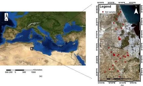
Gabes-Ghannouch is both a Mediterranean and Saharan region. It is located in
South-Eastern Tunisia from Jeffara plain into the Gulf of Gabes (Figure 1(a)).
The study area has been chosen not only because of the important agriculture in-terests in this region, but also the environmental problems related to soil, such as salinization. Geographic location corresponds to a Latitude/Longitude respectively
DOI: 10.4236/ars.2019.83005 80 Advances in Remote Sensing Figure 1. Location of the study area (a) Composed MODIS image of Mediterranean sea from 2005 (b) Sentinel_2 image of south-ern Tunisia 2018.
where maximum temperatures reached in the period between June and August (48˚C), while the coldest temperatures are measured between December and February. Due to its proximity to the sea, the climate of the study area slightly differs from the typical arid or semi-arid. The rainfall is irregular and ranges between 150 - 240 mm per year with six months dry season (April-Sept), where the rain does not exceed 4 mm per month.
According to [32] the investigated area is situated under an arid climate,
where the annual evaporation value is ~1950 mm using the Pische and Bac me-thods. The evaporation in this region is relatively very high due to the dry cli-mate conditions; therefore salt left after water evaporation on the top soils ac-cumulates rapidly and accelerates the soil salinization process. This fact leads to salt accumulation in the upper layers of the Chott sediments and to crust forma-tion [33].
The study area includes wetlands and steppe plains as well as areas used for agriculture.
2.2. Soil Sampling Method
DOI: 10.4236/ars.2019.83005 81 Advances in Remote Sensing time; Salt in the soils, in dry season, is rising up due to capillarity. The signal of salty soil, at this period of the year, is stronger and easier to detect from the
opt-ical sensors [34]. The soil sample locations were selected in such a way to
mi-nimize any noise that could affect the spectral signature from the soil. Thus, all samples used in this study are at least 60 m away from objects, which are not de-fined as soil (e.g.: trees, houses, streets, etc.).
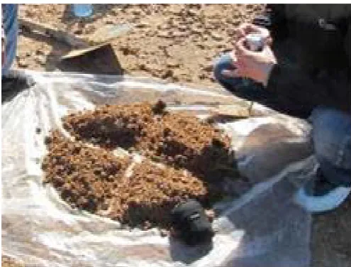
At all sample location, a procedure is used to collect the soil. Each analysed sample in this work is a mix of four soil samples. These 4 samples are collected from 4 corners of a (60 × 60) square, where the center is considered the location of the sample, then the mix of 4 soil collected from 4 corners is the soil sample
considered for chemical analysis Figure 2. These steps are applied for all the
samples, in order to optimize the representation of the samples within the pixel
of the Sentinel_2 image [3]. The use of 60 × 60 m square for the samples
collec-tion aims to be correlated to the spatial resolucollec-tion of the multispectral image. Salinity at the top-soil is determined by measuring electrical conductivity
(EC). 1/5 soil/water diluted extracts is a convenient method [1] used in this
study to estimate soil salt content. To measure the EC of our samples, following steps are conducted: 1) Drying the samples, 2) Sieving (Size of the soil particle <2 mm), 3) Agitation, 4) and then measuring the EC values. EC is usually ex-pressed in decisiemens per m at 25˚C (dS/m).
2.3. Data Used and Statistical Data Processing
The satellite image Sentinel 2 was used to map the soil salinity. This image was acquired in May 2018 and is composed of a multi-spectral imager MSI which provides views in 13 spectral bands from visible to infrared with a resolution va-rying from 10 to 60 meters. Sentinel 2 spectral bands are incorporated into a spectrum range varying from 443 nm (blue) to 2190 nm in the SWIR.
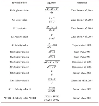
[image:5.595.248.496.503.691.2]Bands reflectance, considered as a spectral indices, and the spectral salinity
DOI: 10.4236/ars.2019.83005 82 Advances in Remote Sensing indices derived from the blue, green, red and near infra-red bands, were used to predict soil salinity from satellite images. After obtaining these indices from the Sentinel_2 image corresponding to the sampling sites, correlation analyzes be-tween the EC measurements and these indices were performed, these
correla-tions are based on the Pearson function. The indices are described in Table 1.
Statistical method is performed like multiple regression models. The purpose is to understand the relation between the spectral indices and the electrical con-ductivity of sampled soil.
2.4. Linear Regression Model
A linear regression was used to establish relationship between the NIR, SWIR spectra and the reference data from analysis of EC based on the statistical
analy-sis. The highest values of R2 and the lowest value of RMSE (root mean square
[image:6.595.203.540.374.733.2]error) were used to determine the optimal calibrated model. The smallest RMSE indicate the most accurate prediction, this RMSE was derived according to equal of (1). The model will be assessed graphically by analysing the standardized re-siduals versus the predicted values of EC. By plotting the rere-siduals with the de-scriptive variable, if a trend is identified, it indicates that the model is not accurate
Table 1. Formula used to generate the indices.
Spectral indices Equation References
BI: Brightness index 2 2 2
3
B G+ +R Zhuo Luoa et al., 2008
CI: Color index R G
R G
−
+ Zhuo Luoa et al., 2008
HI: Hue index 2R G BG B− −− Zhuo Luoa et al., 2008
RI: Redness index 2 2
R
B G+ Zhuo Luoa et al., 2008
SI: Salinity index R 100
NIR× Tripathi et al., 1997
SI1: Salinity index 1 B R∗ Khan et al., 2005
SI2: Salinity index 2 G R∗ Khan et al., 2005
SI3: Salinity index 3 G2+R2+NIR2 Douaoui et al., 2006
SI4: Salinity index 4 G2+R2 Douaoui et al., 2006
SI5: Salinity index 5 BR Bannari et al., 2008
SI9: salinity index 9 NIR R
G
− Abass and Khan, 2007
SI-11: Salinity index 11 1
2
SWIR
SWIR Bannari et al., 2008
ASTER_SI: Salinity index ASTER 1 2
1 2
SWIR SWIR SWIR SWIR
−
DOI: 10.4236/ars.2019.83005 83 Advances in Remote Sensing and there is an autocorrelation in the residuals, which is contrary to one of the assumptions of parametric linear regression.
( )
( )
*
1 1
RMSE N Z xi Z xi 2
N
=
∑
− (1)where: N; Number of points, Z*(xi) is estimated value at point xiZ(xi) and is
ob-servation value at point xi.
3. Result and Discussion
Based on the data set collected from the fieldwork, the investigation area is con-sidered as highly affected by salinity according to the results obtained from the
Department of primary industries in Australia [35]. The study area is also
dom-inated by a gypsic soil [9]. These areas of high and extreme saline soil are
com-pletely degraded region, where plants growth is suppressed. Alike Halophyte plants, which are very rare to find and it is very hard to grow through the high content of gypsum [4].
3.1. Descriptive Analysis
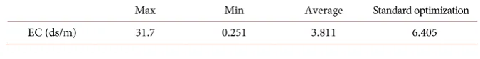
The main statistical parameters for EC data are given in Table 2. The
distribu-tion of the EC values is characterized by an average of 3.81 dS/m and a standard deviation of 6.40. A significant difference between a minimum of 0.25 dS/m (EC of healthy soils) and a maximum of 31.7 dS m (EC of saline soils), which reflects a significant spatial variability of this component [36].
3.2. Correlation between Spectral Indices and EC from the
Ground Truth
A Pearson correlation between the electrical conductivity values and the Sentinel
2 spectral bands was conducted Table 1 to evaluate which spectrum interval
could reveal more about the salt affected area. Correlation between the Sentinel 2 spectral bands and EC from the ground truth shows a higher correlation in the
SWIR region of the spectrum interval as shown in Table 3.
The most correlated bands are the band 11 and 12 of SWIR, the empiric equa-tion A = log(1/R) which transform the reflectance to absorbance improve the correlation by 3% that’s why bands absorbance will be considered as spectral in-dices and will be integrated to construct the model. The salinity index SI
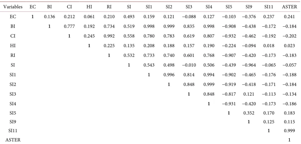
pro-vides the highest correlation 49% Table 4, not only among the salinity indices
but among all the spectral indices performed in this work.
[image:7.595.202.540.694.736.2]Color indices showed a low correlation with EC varying between 13% and 21%. Salinity indices show a moderate correlation with the EC, varying between 8% and 49%.
Table 2. Descriptive statistics on the electrical conductivity of samples.
Max Min Average Standard optimization
DOI: 10.4236/ars.2019.83005 84 Advances in Remote Sensing Table 3. Correlation matrix between Landsat spectral bands and EC values.
Variables EC band2 band3 band4 band8 band11 band12
EC 1 0.172 0.083 0.145 −0.232 −0.409 −0.436
band2 1 0.956 0.859 0.454 0.542 0.497
band3 1 0.942 0.630 0.627 0.570
band4 1 0.610 0.610 0.569
band8 1 0.520 0.474
band11 1 0.934
band12 1
Table 4. Correlation matrix between salinity indices and EC values.
Variables EC BI CI HI RI SI SI1 SI2 SI3 SI4 SI5 SI9 SI11 ASTER
EC 1 0.136 0.212 0.061 0.210 0.493 0.159 0.121 −0.088 0.127 −0.103 −0.376 0.237 0.241
BI 1 0.777 0.192 0.734 0.519 0.998 0.999 0.835 0.998 −0.908 −0.438 −0.172 −0.184
CI 1 0.245 0.992 0.558 0.780 0.783 0.619 0.807 −0.932 −0.462 −0.192 −0.202
HI 1 0.225 0.135 0.208 0.188 0.157 0.190 −0.224 −0.094 0.018 0.023
RI 1 0.532 0.733 0.740 0.601 0.768 −0.907 −0.420 −0.173 −0.183
SI 1 0.543 0.498 −0.010 0.506 −0.439 −0.964 −0.065 −0.057
SI1 1 0.996 0.814 0.994 −0.902 −0.465 −0.176 −0.188
SI2 1 0.848 0.999 −0.919 −0.418 −0.171 −0.184
SI3 1 0.848 −0.817 0.121 −0.113 −0.134
SI4 1 −0.931 −0.420 −0.173 −0.186
SI5 1 0.352 0.170 0.183
SI9 1 0.125 0.115
SI11 1 0.999
ASTER 1
The most correlated is spectral salinity index SI Table 4 and SWIR bands (b11
and b12).
3.3. Regression Analysis Modelling
The linear regression is used to predict the spatial variability of soil salinity based on remote sensing and ground truth measurements. The prediction of the EC values from Sentinel_2 bands and the spectral indices is associated with the identification of 3 variables shown in Equation (2). A significant coefficient of
determination R2 indicates that the predictor variables used in the model can
ex-plain 48% of the total variation of the predicted EC values. The regression em-pirical relationship is given by the following formula:
EC= −0.3 0.4 SI 5.2E 03 band11 4.9E 03 band12+ × − − × − − × (2)
[image:8.595.57.540.245.477.2]DOI: 10.4236/ars.2019.83005 85 Advances in Remote Sensing to the ground truth measurement.
The empirical relationship between measured and estimated EC values showed
an overestimation of the predicted electrical conductivity values. Figure 3 shows
that predicted values of electrical conductivity are often higher than the values from the ground truth measurements.
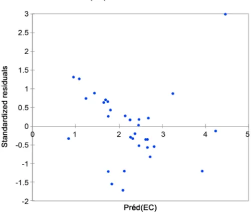
[image:9.595.249.498.206.426.2]The plot of the standardized residuals versus the predicted values of EC shown in Figure 4 proved that no specific trends are identified; therefore, our proposed regression model is approved.
Figure 3. Relationship between measured and estimated electrical conductivity values.
[image:9.595.248.499.483.695.2]DOI: 10.4236/ars.2019.83005 86 Advances in Remote Sensing
4. Conclusions
The present study demonstrates that combining the Sentinel_2 SWIR bands and the salinity index into a regression model offers a potentially quick and inexpen-sive method to model the spatial variation in soil salinity. The combination of these remotely sensed variables into one model was able to explain 48% of the spatial variation in the soil salinity of the study area.
Although this study demonstrates that soil salinity mapping and modelling can be undertaken with good accuracy based on high spatial resolution multis-pectral images, further research is needed to focus on investigating the possibili-ty of hyperspectral data in mapping and modelling soil salinipossibili-ty.
Conflicts of Interest
The authors declare no conflicts of interest regarding the publication of this pa-per.
References
[1] Department of Primary Industries (1996) Victorian Resources Online.
http://www.dpi.vic.gov.au
[2] Lu, D. and Weng, Q. (2005) Urban Classification Using Full Spectral Information of LANDSAT ETM+ Imagery in Marion County, Indiana. Photogrammetric Engi-neering and Remote Sensing, 71, 1275.https://doi.org/10.14358/PERS.71.11.1275
[3] Weng, Y., Gong, P. and Zhu, Z. (2008) Reflectance Spectroscopy for the Assessment of Soil Salt Content in Soils of the Yellow River Delta of China. International Jour-nal of Remote Sensing, 29, 5511-5531.https://doi.org/10.1080/01431160801930248
[4] Gueddari, M., Monnin, C., Perret, D., Fritz, B. and Tardy, Y. (1983) Geochemistry of Brines of the Chott el Jerid in Southern Tunisia—Application of Pitzers Equa-tions. Chemical Geology, 39, 165.https://doi.org/10.1016/0009-2541(83)90078-5
[5] Congalton, R. and Green, K. (2009) Assessing the Accuracy of Remote Sensed Data: Principles and Practices. 2nd Edition, CRC/Lewis Press, Boca Raton, 137.
https://doi.org/10.1201/9781420055139
[6] Triki, I., Trabelsi, N., Zairi, M. and Ben Dhia, H. (2013) Multivariate Statistical and Geostatistical Techniques for Assessing Groundwater Salinization in Sfax, a Coastal Region of Eastern Tunisia. Desalination and Water Treatment, 52, 1980-1989.
https://doi.org/10.1080/19443994.2013.803937
[7] Tóth, T., Pasztor, L., Kabos, S. and Kuti, L. (2002) Statistical Prediction of the Pres-ence of Salt-Affected Soils by Using Digitalized Hydrogeological Maps. Arid Land Research and Management, 16, 55-68.
https://doi.org/10.1080/153249802753365322
[8] Shrestha, D., Margateb, D.E., van der Meer, F. and Anhc, H.V. (2005) Analysis and Classification of Hyperspectral Data for Mapping Land Degradation: An Applica-tion in Southern Spain. International Journal of Applied Earth Observation and Geoinformation, 7, 85.https://doi.org/10.1016/j.jag.2005.01.001
[9] Wang, H., Wang, J. and Liu, G. (2007) Spatial Regression Analysis on the Variation of Soil Salinity in the Yellow River Delta. Proceedings of the SPIE 6753, Geoinfor-matics 2007: Geospatial Information Science, Nanjing, 10 June 2007, 67531U.
DOI: 10.4236/ars.2019.83005 87 Advances in Remote Sensing
[10] Jobson, J.D. (1999) Applied Multivariate Data Analysis: Volume 1: Regression and Experimental Design. Springer Verlag, New York.
[11] Metternicht, G. and Zinck, A. (2008) Remote Sensing of Soil Salinization: Impact on Land Management. CRC Press, Boca Raton, 377.
https://doi.org/10.1201/9781420065039
[12] Farifteh, J., van der Meer, F., Atzberger, C. and Carranza, E. (2007) Quantitative Analysis of Salt-Affected Soil Reflectance Spectra: A Comparison of Two Adaptive Methods (PLSR and ANN). Remote Sensing of Environment, 110, 59-78.
https://doi.org/10.1016/j.rse.2007.02.005
[13] Fethi, B., Magnus, P., Ronny, B. and Akissa, B. (2010) Estimating Soil Salinity over a Shallow Saline Water Table in Semiarid Tunisia. The Open Hydrology Journal, 4, 91-101.https://doi.org/10.2174/1874378101004010091
[14] Taghizadeh-Mehrjardi, R., Minasny, B., Sarmadian, F. and Malone, B. (2014) Digi-tal Mapping of Soil Salinity in Ardakan Region, Central Iran. Geoderma, 213, 15-28.
https://doi.org/10.1016/j.geoderma.2013.07.020
[15] Malins, D. and Metternicht, G. (2006) Assessing the Spatial Extent of Dryland Sa-linity through Fuzzy Modeling. Ecological Modelling, 193, 387-411.
https://doi.org/10.1016/j.ecolmodel.2005.08.044
[16] Douaik, A., van Meirvenne, M., Toth, T. and Serre, M. (2004) Space-Time Mapping of Soil Salinity Using Probabilistic Bayesian Maximum Entropy. Stochastic Envi-ronmental Research and Risk Assessment, 18, 219-227.
https://doi.org/10.1007/s00477-004-0177-5
[17] Triantafilis, J., Odeh, I. and McBratney, A. (2001) Five Geostatistical Models to Pre-dict Soil Salinity from Electromagnetic Induction Data across Irrigated Cotton. Soil Science Society of America Journal, 65, 869-878.
https://doi.org/10.2136/sssaj2001.653869x
[18] Fan, X., Pedroli, B., Liu, G., Liu, Q., Liu, H. and Shu, L. (2012) Soil Salinity Devel-opment in the Yellow River Delta in Relation to Groundwater Dynamics. Land De-gradation & Development, 23, 175-189.https://doi.org/10.1002/ldr.1071
[19] Eldeiry, A.A. and Garcia, L.A. (2008) Detecting Soil Salinity in Alfalfa Fields Using Spatial Modeling and Remote Sensing. Soil Science Society of America Journal, 72, 201-211.https://doi.org/10.2136/sssaj2007.0013
[20] McBratney, A., Santos, M.D.L.M. and Minasny, B. (2003) On Digital Soil Mapping.
Geoderma, 117, 3-52.https://doi.org/10.1016/S0016-7061(03)00223-4
[21] Scull, P., Franklin, J., Chadwick, O. and McArthur, D. (2003) Predictive Soil Map-ping: A Review. Progress in Physical Geography, 27, 171-197.
https://doi.org/10.1191/0309133303pp366ra
[22] Lesch, S.M., Strauss, D.J. and Rhoades, J.D. (1995) Spatial Prediction of Soil Salinity Using Electromagnetic Induction Techniques: 1. Statistical Prediction Models: A Comparison of Multiple Linear Regression and Cokriging. Water Resources Re-search, 31, 373-386.https://doi.org/10.1029/94WR02179
[23] Thomas, D.S.G. and Middleton, N.J. (1993) Salinization: New Perspectives on a Major Desertification Issue. Journal of Arid Environments, 24, 95.
https://doi.org/10.1006/jare.1993.1008
[24] Douaoui, A.E.K., Nicolas, H. and Walter, C. (2006) Detecting Salinity Hazards within a Semiarid Context by Means of Combining Soil and Remote-Sensing Data.
Geoderma, 134, 217-230.https://doi.org/10.1016/j.geoderma.2005.10.009
DOI: 10.4236/ars.2019.83005 88 Advances in Remote Sensing
Valley, Mexico: Application of a Practical Method for Agricultural Monitoring.
En-vironmental Management, 50, 478-489.https://doi.org/10.1007/s00267-012-9889-3
[26] Qu, Y.H., Jiao, S.O. and Lin, X.D. (2008) A Partial Least Square Regression Method to Quantitatively Retrieve Soil Salinity Using Hyper-Spectral Reflectance Data. Pro-ceedings of the SPIE 7147, Geoinformatics 2008 and Joint Conference on GIS and Built Environment: Classification of Remote Sensing Images, Guangzhou, 31 Octo-ber 2008, 71471H.
[27] Shamsi, F.R.S., Sanaz, Z. and Abtahi, A.S. (2013) Soil Salinity Characteristics Using Moderate Resolution Imaging Spectroradiometer (MODIS) Images and Statistical Analysis. Archives of Agronomy and Soil Science, 59, 471-489.
https://doi.org/10.1080/03650340.2011.646996
[28] Mehrjardi, R.T., Mahmoodi, S.H., Taze, M. and Sahebjalal, E. (2008) Accuracy As-sessment of Soil Salinity Map in Yazd-Ardakan Plain, Central Iran, Based on Land-sat ETM+ Imagery. American-Eurasian Journal of Agricultural & Environmental Sciences, 3, 708-712.
[29] Tajgardan, T., Shataee, S. and Ayoubi, S. (2007) Spatial Prediction of Soil Salinity in the Arid Zones Using ASTER Data, Case study: North of Ag Ghala, Golestan Prov-ince, Iran. Proceedings of Asian Conference on Remote Sensing, Kuala Lumpur, 12-16 November 2007.
[30] Afework, M. (2009) Analysis and Mapping of Soil Salinity Levels in Metehara Su-garcane Estate Irrigation Farm Using Different Models. Ms.C. Thesis, Addis Ababa University, Addis Ababa.
[31] Bouaziz, M., Matschullat, J. and Gloaguen, R. (2011) Improved Remote Sensing Detection of Soil Salinity from a Semi-Arid Climate in Northeast Brazil. Comptes Rendus Geoscience, 343, 795-803.https://doi.org/10.1016/j.crte.2011.09.003
[32] Szabolcs, I. (1989) Salt Affected Soils. CRC Press, Boca Raton.
[33] Wu, T.N., Huang, Y.C., Lee, M.S. and Kao, C.M. (2005) Source Identification of Groundwater Pollution with the Aid of Multivariate Statistical Analysis. Water Science and Technology: Water Supply, 5, 281-288.
https://doi.org/10.2166/ws.2005.0074
[34] Dutkiewicz, A., Lewis, M. and Ostendorf, B. (2009) Evaluation and Comparison of Hyperspectral Imagery for Mapping Surface Symptoms of Dry Land Salinity. Inter-national Journal of Remote Sensing, 30, 693.
https://doi.org/10.1080/01431160802392612
[35] Dehaan, R.L. and Taylor, G.R. (2002) Field-Derived Spectra of Salinized Soils and Vegetation as Indicators of Irrigation-Induced Soil Salinization. Remote Sensing of Environment, 80, 406.https://doi.org/10.1016/S0034-4257(01)00321-2
[36] Liu, C.-W., Lin, K.-H. and Kuo, Y.-M. (2003) Application of Factor Analysis in the Assessment of Groundwater Quality in a Blackfoot Disease Area in Taiwan. The Science of the Total Environment, 313, 77-89.