Solar Thermal Aquaculture System Controller Based on Artificial Neural Network

Engineering, 2011, 3, 815-822

doi:10.4236/eng.2011.38099 Published Online August 2011 (http://www.SciRP.org/journal/eng)

Solar Thermal Aquaculture System Controller Based on

Artificial Neural Network

Doaa M. Atia1, Faten H. Fahmy1, Ninet M. Ahmed1, Hassen T. Dorrah2

1_{Electronics Research Institute, Cairo, Egypt}

2_{Electrical Power and Machines, Faculty of Engineering,Cairo Univ. Cairo, Egypt} E-mail: [email protected]

ReceivedDecember 16, 2010; revised July 5, 2011; accepted July 15, 2011

Abstract

Temperature is one of the most principle factors affects aquaculture system. The water temperature is very important parameter for shrimp growth. It can cause stress and mortality or superior environment for growth and reproduction. The required temperature for optimal growth is 34˚C, if temperature increase up to 38˚C it causes death of the shrimp, so it is important to control water temperature. Solar thermal water heating sys-tem is designed to supply an aquaculture pond with the required hot water in Mersa Matruh in Egypt as pre-sented in this paper. This paper introduces a complete mathematical modeling and MATLAB SIMULINK model for the solar thermal aquaculture system. Moreover the paper presents the control of pond water tem-perature using artificial intelligence technique. Neural networks are massively parallel processors that have the ability to learn patterns through a training experience. Because of this feature, they are often well suited for modeling complex and non-linear processes such as those commonly found in the heating system. They have been used to solve complicated practical problems. The simulation results indicate that, the control unit success in keeping water temperature constant at the desired temperature by controlling the hot water flow rate.

Keywords:Aquaculture, Forced Circulation Hot Water System, Artificial Neural Networks

1. Introduction

The shrimp farming is an important economical activity in many countries [1]. Intensive aquaculture is a modern cultivation way and it develops fast in many countries. Recently, People pay more and more attention on aqua-culture for its advantages of high yield, no-time-limit, low-feed and high-utilization of water [2]. The purpose for applying process control technology to aquaculture in developed countries encompasses many socioeconomic factors, including variable climate. Anticipated benefits for aquaculture process control systems are to be in-creased process efficiency, reduced energy and water losses, reduced labor costs, reduced stress and disease, improved accounting, improved understanding of the process [3].

The study of artificial neural networks (ANN) is one of the two major branches of intelligence control, which is based on the concept of artificial intelligence (AI). AI can be defined as computer emulation of the human thinking process. During the last ten years, there has been

a substantial increase in the interest on artificial neural networks. During the last ten years, there has been a sub-stantial increase in the interest on artificial neural net-works. The ANNs are good for some tasks while lacking in some others. Specifically, they are good for tasks in-volving incomplete data sets, fuzzy or incomplete infor-mation and for highly complex and ill-defined problems, where humans usually decide on an intuitional basis [4-6]. In this paper the control of water temperature of aquaculture system is achieved. ANN control is chosen to this task due to high efficiency in control application.

2. Mathematical Model of Solar Thermal

System

Storage tank temperature is an important parameter which influences the system size and performance. Energy bal-ance of a well mixed storage tank can be expressed as [7]

d

d st

s p c l

T

V c q q q

t

where  water density (kg/m3), Vs isis storage tank

vol-ume (m3), Tstis storage tank temperature (˚C), Cp is

spe-cific heat of water (4190 J/kg·˚C), qcis actual useful

en-ergy gain, ql is load energy, and qstl is storage tank losses.

2.1. Flat Plate Collector Modeling

Solar useful heat gain rate (qc) from the collector array is

calculated by





c R c l i a

q F A _G U T T  _ (2) where qc represents actual usefulenergy gain (W),FRthe

collector heat removal factor, G intensity of solar radia-tion, in (W/m2), Ac collector surface area (m2), (α) is the

transmittance absorptance product, Ulis collector overall

heat transfer coefficient (W/m2·˚C), Ta is the ambient

temperature (˚C), and Ti is the inlet temperature. Where

+ sign indicates that only positive values of qc is

consid-ered in the analysis. This implies that hot water from the collector enters the tank only when solar useful heat gain becomes positive [7].

2.2. Mathematical Modeling of the Aquaculture Pond

A numerical model based on energy balance was devel-oped to simulate the thermal behavior of the open-pond system. Assumed uniform temperature for the entire pond, and thus applied a well-mixed model [8].

2.2.1. Evaporation Losses

The evaporation heat loss is the largest loss component and is given



 

e p a p a p a

q A P_ V T T _  



  (3)

where qe is the evaporation loss (W), V is the wind speed

in (m/s) in the vicinity of the pond, Pa the ambient air

pressure (101.3 k·Pa). TP is the pond temperature, Ta is

the ambient temperature, ωP is the saturation humidity

ratio at the pond temperature, ωa is the humidity ratio of

the ambient air above the pond, Ap is the area of the pond

[8,9].

2.2.2. Convection Losses

Heat losses due to convection to the ambient air can be expressed as [8,9]

0.0006 p a

c e

p a

T T

q q

 

  

 (4)

2.2.3. The Net Radiation Losses

Results from the surface of the pond to the sky which can be expressed as [8,9]:





4

273

r p p

q  A _T  Ts _ (5)

where qr is the radiation loss, ε is the emissivity of the

surface, σ is the Stefan-Boltzmann constant, TS is the sky

temperature in degrees Kelvin, Tp is the pond

tempera-ture.

2.2.4. Solar Radiation Heat Gain

Heat gain due to the absorption of solar radiation by the pond is given by [8,9]

s p

q A G (6) where  is pond absorptance (0.9).

2.3. The Control Thermostatic Valve Modeling

The required characteristic of this valve must be linear, such that controlling the valve input signal, will directly control the mass flow rate of water. Therefore, the trans-fer function of the used valve will be considered to be a first order one, as

 

v

G s s



 (7)

3. Required Pond Design

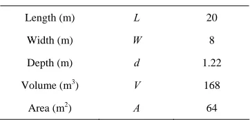
The pond is selected to be a rectangular shape as shown in Figure 1. The parameters of the pond are indicated in

Table 1.

L

W

(a)

1.22 m 2 m

(b)

Figure 1. Pond design (a) Pond dimension; (b) Pond cross section detail.

Table 1. The pond dimension.

Length (m) L 20

Width (m) W 8

Depth (m) d 1.22

Volume (m3_{) V 168}

D. M. ATIA ET AL. ₈₁₇

4. Neura

rk Desc ption

en suggested for

l Netwo

ri

n recent years, neural solutions have be I

many industrial systems using either feed-forward or recurrent neural networks. The ANN is usually made up of activation function neurons and training algorithm is normally used to train the network either online or off- line. Some applications use neurons with a radial base activation function. The ANN may play different roles: plant identification, non-linear controller, and fault sig-naling. Typical neural networks used for identification purposes are multilayer feed-forward structures contain-ing neurons with activation function. There are two con-figurations for plant identification: the forward configu-ration and the inverse configuconfigu-ration [10-12]. A neural network consists of a number of processing elements “neurons” each of which have many inputs but only one output. In a typical network there are three layers of neurons, which are input layer receives input from the outside world, hidden layer which receive inputs from the input layer neurons and the output layer which re-ceives inputs from the hidden layers and passes its output to the outside world and in some cases back to the pre-ceding layers. In a feed forward neural network, the value of each node in a particular hidden layer is the re-sult of a non linear transfer function a whose argument is the weighted sum over all the nodes in the previous layer plus a constant term b which is referred to as the bias as presents in Equation (8)

i j ij

j

x 



The j subscript refers to a summatio th

8)

n of all nodes in e previous layer of nodes and the i subscript refers to the node position in the present layer. In order to solve for the weight and bias values of Equation (8) for all nodes, one requires a set of input patterns, representative of the system behavior. A variety of training algorithms are available but in general, to train a network, one be-gins with a set of training data consisting of the input vector, and corresponding target vector. The internal weights are adjusted until the sum of differences between the neural network outputs and the corresponding target is minimized to a pre-determined level for all the training data. A sigmoidal function is usually used for the transfer function as it enables a finite number of nodes in a single hidden layer to uniformly approximate any continuous function

1 1 e

j xj

y  _

 (9)

.1. The Error Back-Propagation Algorithm

the

ne named “error back-propagation”, or simply “back-

4

The most popular supervised training algorithm is

o

propagation”. It involves training a FFANN structure made up of activation function neurons. The back-pro- pagation algorithm is a gradient method aiming to mini-mize the total operation error of the neural network. The process is intended to minimize the Error between the network output and the output actual output for the same input. The total error is a function defined by

2 1

2 j j

RMS



j

(10)

where t is target value, and o is output

ormation patterns within a multi dimensional information domain.

rep-d

vari-to learn

al methods.

ide the system with e required control action. Thermostatic valve is used to

ontrol

rol after many trials, shown in

igure 3, eventually employed three layers which are the value [10-14].

4.2. Neural Network Advantages

 ANNs are able to learn the key inf

 The inherently noisy data do not seem to cause a problem, since they are neglected. ANN models resent a new method in system prediction.

 ANNs operate like a black box model and do not re-quire detailed information about the system.

 Instead, they learn the relationship between the input parameters and the controlled and uncontrolle ables by studying previously recorded data, similar to the way a non linear regression might perform.

 ANNs has the ability to handle large and complex systems with many interrelated parameters.

 Artificial neural networks differ from traditional si- mulation approaches in that they are trained

solutions rather than being programmed to model a specific problem in the normal way.

 They are used to address problems that are intractable or cumbersome to solve with tradition

5. Proposed Control System

The neural network is utilized to prov th

adjust the hot water mass flow rate through the system to control the pond temperature at 34oC. The proposed con-trol system consists of the ANN concon-troller which is used to control water temperature. The control signal is used to control the operation of thermostatic valve to control the hot water flow rate added to the pond as depicted in

Figure 2.

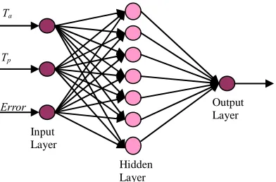
6. ANN C

The proposed NN cont

F

con-Ta

Tp

Error Output

Layer

Hidden Layer Input

Layer

sists of seven neurones, and output layer of one neurons as shown in Figure 3. The activation function used in this work is “logsig” for hidden layer, and “purelin” for output layer. The NN is trained using a back propagation with Levenberg-Marquardt algorithm. The Back propa-gation is a form of supervised learning for multi-layer nets. Error data at the output layer is back propagated to earlier ones, allowing incoming weights to these layers to be updated. It is most often used as training algorithm in current neural network applications. Figure 4 presents the mean square error between the network output and the target. The network response analysis is depicted in

Figure 5. As shown in the figure the regression “R” equal one which mean the output track the target in a correct way.

Figure 3. Neural network controller architecture.



Tp

e

NN Controller

Thermostatic

valve Pond

Ta

Tp

+ Tref

Tp

Cs mw

Figure 2. Block diagram of pond temperature control using

NN control. Figure 4. Mean square error.

D. M. ATIA ET AL. ₈₁₉

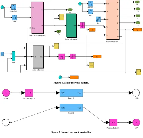
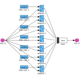
7. System Simulation

The simulation model of the proposed thermal system is depicted in Figure 6. The system consists of solar ther-mal subsystem to feed the system with the required hot water during the day, biogas subsystem is the auxiliary heater, pond subsystem, and finally the control subsys-tem. MATLAB SIMULINK of NNC is depicted in Fig-ure 7. Figure 8 indicates the weight block diagram of layer1.

8. Results and Discussion

The results of the MATLAB software indicate the high

capability of the proposed technique in controlling the water temperature in the aquaculture pond, even in case of changing atmospheric conditions. The system has two input parameters they are air temperature, and solar ir-radiance. Figure 9 and Figure 10 represent solar irradi-ance in Mersa Matruh the site of consideration in sum-mer and winter respectively. Figures 11 and 12 show the air temperature in summer and winter.

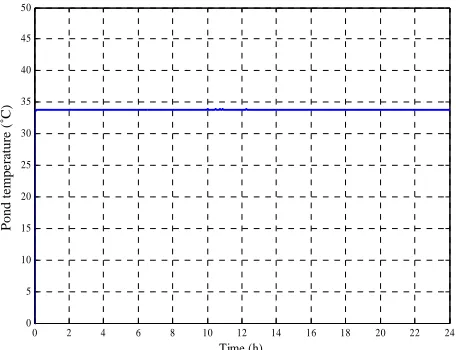
Figures 13 and 14 indicate the pond temperature in summer and winter respectively. It is shown that the NN control has adjust the water temperature at 34˚C without any variation during the day. Any variation in water tem- perature will harm the shrimp life, so the NN control has successes in this process.

Ts 6

qu 5

qc 4 qr 3 qs 2 qe 1

solar therma

Rad

Ta

qload qu

Ts

l subsystem

Rad

Ta

RH

Th

qe

qs

qr

qc

Tp

pond Subsystem

m

ql

control subsystem

x{1} y{1} 1

s+1

t

Thw

mw

Tp Tair1

Tair

Solar Rad 1 Solar Rad

RH

34

Biogas subsy

T Twh

stem

Add

rmal system. Figure 6. Solar the

1

Process Output 1 a y Process Input 1

x p

Layer 1 a {1} 1

x {1}

p {1}

Layer 2

a {1} a {2}

a {1}

y {1}

iz{1,1} 1 dotprod 7 w p z dotprod 6 w p z dotprod 5 w p z dotprod 4 w p z dotprod 3 w p z dotprod 2 w p z dotprod 1 w p z Mux Mux IW{1,1}(7,:)' weights IW{1,1}(6,:)' weights IW{1,1}(5,:)' weights IW{1,1}(4,:)' weights IW{1,1}(3,:)' weights IW{1,1}(2,:)' weights IW{1,1}(1,:)' weights pd {1,1} 1

Figure 8. Block diagram of layer 1 weights.

0 2 4 6 8 10 12 14 16 18 20 22 24 0 100 200 300 400 500 600 700 800 900 1000 Time (h) S o la r ir ra d ia n ce ( W /m 2 ) S lol ar i rr adi ance ( W /m 2)

0 2 4 6 8 10 12 14 16 18 20 22 24 0 100 200 300 400 500 600 700 800 1000 900 Time (h) S o la r i rra di an ce (W /m 2)

Figure 9. Solar irradiance in summer.

S lol ar i rr adi ance ( W /m 2)

Figure 10. Solar irradiance in winter.

0 2 4 6 8 10 12 14 16 18 20 22 24 0 5 10 15 20 25 30 Time (h) A ir tem p er atu re (o C ) Ai r t em p er at ur e ( ˚C)

0 2 4 6 8 10 12 14 16 18 20 22 24 0 5 10 15 20 25 30 Time (h) A ir t em p er atu re (o C ) Ai r t em p e rat ur e ( ˚C)

D. M. ATIA ET AL. ₈₂₁

0 2 4 6 8 10 12 14 16 18 20 22 24

0 5 10 15 20 25 30 35 40 45 50 Time (h) P o nd t em p er at ur e ( o C ) Pond tempe rature ( ˚C)

0 2 4 6 8 10 12 14 16 18 20 22 24 0 5 10 15 20 25 30 35 40 45 50 Time (h) P ond t em pe ra ture ( o C ) Pond tempe rature ( ˚C)

Figure 13. Pond temperature (˚C) in summer. Figure 14. Pond temperature (˚C) in winter.

0 2 4 6 8 10 12 14 16 18 20 22 24 0 2 4 6 8 10 12 14 16 18 20 22 24 26 Time (h) M as s fl o w ra te (K gp h)

0 2 4 6 8 10 12 14 16 18 20 22 24 0 2 4 6 8 10 12 14 16 26

Figure 15. Mass flow rate in summer.

18 20 22 24 Time (h) M as s fl o w ra te () M as s f low ra te (K gph)

Figure 16. Mass flow rate in winter.

Figures 15 and 16 show the hot water flow rate varia-tion over the day in summer and winter respectively. It i

clear that

tempera-ture increase ses.

uring the night hours the mass flow rate has high value rather than that the day hours. The mass flow rate in winter is higher than in summer because of low air tem-perature in winter than in summer. The simulation results show the high efficiency of the proposed control system in control pond water temperature.

9. Conclusiona

The most important parameters to be monitored and con-trolled in an aquaculture system are related to water quality, since they directly affect animal health. Neural networks offer one such method with their ability to map complex nonlinear functions. Neural networks are mas-sively parallel processors that have the ability to learn

patterns t e of this

feature, they are often well suited for modeling complex and non-linear processes such as those commonly foun

in the he the NN

technique to con uaculture

pond. The air temperature, pond temperature, and error are used as inputs to NN control. Offline training applied with the BP has been used. The simulation results show that the feasibility of NN control in keeping water tem-perature constant at the desired degree (34˚C) by adjust the mass flow rate of hot water to the pond.

10. References

[1] J. J. Carbajal1 and L. P. Sanchez, “Classification Based on Fuzzy Inference Systems for Artificial Habitat Quality in Shrimp Farming,” In Proceedings of IEEE Conference 7th Mexican International on Artificial Intelligence, Pachuca, 27-31 October 2008, pp. 388-392.

[2] X. J. Shena, M. Chena and J. Yub, “Water Environment Monitoring System Based on Neural Networks fo

Shrim E

Interna-s as air temperature increase the pond

, so the value of mass flow rate decrea D

hrough a training experience. Becaus

d ating system. This paper introduces

trol the water temperature of aq

tional Conference on Artificial Intelligence and Compu-tational Intelligence, Vol. 3, 2009, pp. 427-431.

[3] P. G. Lee, “Process Control and Artificial Intelligence Software for Aquaculture,” Aquacultural Engineering, Vol. 23, No. 1-3, 2000, pp. 13-36.

doi:10.1016/S0144-8609(00)00044-3

[4] S. A. Kalogeria, “Applications of Artificial Neural Net-works in Energy Systems: A Review,” Energy

Conver-sion & Management, Vol., 40, No. 10, 1999, pp. 1073- 1087. doi:10.1016/S0196-8904(99)00012-6

[5] J. W. Moon, S. K. Jung and J.-J. Kim, “Application of Ann (Artificial-Neural-Network) in Residential Thermal Control,” Building and Simulation, Proceedings of 11th

International IBPSA Conference, Glasgow, 27-30 July 2009.

[6] H. Mirinejad, S. H. Sadati, M. Ghasemian and H. Torab

“ d Air

C puter

Science, Vol. 4, No. 9, 2008, pp. 777-783. doi:10.3844/jcssp.2008.777.783

, Control Techniques in Heating, Ventilating an

onditioning (Hvac) Systems,” Journal of Com

[7] G. N. Kulkarni, S. B. Kedare and S. Bandyopadhyay, “Determination of Design Space and Optimization of So-lar Water Heating Systems,” Solar Energy, Vol. 81, No. 8, 2007, pp. 958-968. doi:10.1016/j.solener.2006.12.003 [8] J. Gelegenis, P. Dalabakis and A. Ilias, “Heating of a Fish

Wintering Pond Using Low-Temperature Geothermal

Fluids, Porto Lagos, Greece,” Geothermics, Vol. 35, No. 1, 2006, pp. 87-103.

doi:10.1016/j.geothermics.2005.10.004

[9] J. Duffie and W. Beckman, “Solar Engineering of Ther-mal Processes,” 2nd Edition, John Wiley & Sons Inter-science, New York, 1991.

[10] S.A Kalogiroua, S. Pantelioub and A. Dentsoras, “Artifi-cial Neural Networks Used for the Performance Predic-tion of a Thermosiphon Solar Water Heater,” Renewable

Energy, Vol. 18, No. 1, 1999, pp. 87-99. doi:10.1016/S0960-1481(98)00787-3

[11] J. A. Freeman and D. M. Skapura, “Neural Networks Algorithms, Applications, and Programming Techniques,” Addison-Wesley Publishing Company, Inc., Paris, 1991.

[12] M. N. Cirstea, A. Dinu, J. G. Khor and M. McCormick, “Neural and Fuzzy Logic Control of Drives and Power Sy

[13] S. A. Kalogirou

formance Parameters Using Artificial Neural Networks,”

Solar Energy, Vol. 80, 2006, pp. 248-259. doi:10.1016/j.solener.2005.03.003

stems,” Replika Press, Delhi, 2002.

, “Prediction of Flat-Plate Collector

Per-[14] A. Sozen, T. Menlik and S. Unvar, “Determination of Efficiency of Flat-Plate Solar Collectors Using Neural Network Approach,” Expert Systems with Applications, Vol., 35, No. 4, 2008, pp. 1533-1539.