Intelligent Biometric Information Management

(1)

doi:10.4236/iim.2010.29060 Published Online September 2010 (http://www.SciRP.org/journal/iim)

Intelligent Biometric Information Management

Harry Wechsler

Department of Computer Science, George Mason University, Fairfax, USA E-mail: wechsler@gmu.edu

Received June 10, 2010; revised July 29, 2010; accepted August 30, 2010.

Abstract

We advance here a novel methodology for robust intelligent biometric information management with infer-ences and predictions made using randomness and complexity concepts. Intelligence refers to learning, adaptation, and functionality, and robustness refers to the ability to handle incomplete and/or corrupt adversarial information, on one side, and image and or device variability, on the other side. The proposed methodology is model-free and non-parametric. It draws support from discriminative methods using likelihood ratios to link at the conceptual level biometrics and forensics. It further links, at the modeling and implementation level, the Bayesian framework, statistical learning theory (SLT) using transduction and semi-supervised learning, and Information Theory (IY) using mutual information. The key concepts supporting the proposed methodology are a) local estimation to facilitate learning and prediction using both labeled and unlabeled data; b) similarity metrics using regularity of patterns, randomness deficiency, and Kolmogorov complexity (similar to MDL) using strangeness/typicality and ranking p-values; and c) the Cover – Hart theorem on the asymptotical performance of k-nearest neighbors approaching the optimal Bayes error. Several topics on biometric inference and prediction related to 1) multi-level and multi-layer data fusion including quality and multi-modal biometrics; 2) score normalization and revision theory; 3) face selection and tracking; and 4) identity management, are described here using an integrated approach that includes transduction and boost-ing for rankboost-ing and sequential fusion/aggregation, respectively, on one side, and active learnboost-ing and change/ outlier/intrusion detection realized using information gain and martingale, respectively, on the other side. The methodology proposed can be mapped to additional types of information beyond biometrics.

Keywords:Authentication, Biometrics, Boosting, Change Detection, Complexity, Cross-Matching, Data Fusion, Ensemble Methods, Forensics, Identity Management, Imposters, Inference, Intelligent Information Management, Margin gain, MDL, Multi-Sensory Integration, Outlier Detection, P-Values, Quality, Randomness, Ranking, Score Normalization, Semi-Supervised Learning, Spectral Clustering, Strangeness, Surveillance, Tracking, Typicality, Transduction

1. Introduction

Information can be viewed as an asset, in general, and resource or commodity, in particular. Information man-agement [using information technology] stands for the “application of management principles to the acquisition, organization, control, alert and dissemination and strate-gic use of information for the effective operation of or-ganizations [including information architectures and management information systems] of all kinds. ‘Informa-tion’ here refers to all types of information of value, whether having their origin inside or outside the organi-zation, including data resources, such as production data; records and files related, for example, to the personnel

(2)

We start with parsing and understanding the meaning of intelligent information management when information refers to biometrics where physical characteristics, e.g., appearance, are used to verify and/or authenticate indi-viduals. Physical appearance and characteristics can include both internal ones, e.g., DNA and iris, and external ones, e.g., face and fingerprints. Behavior, e.g., face expression and gait, and cognitive state, e.g., intent, can fur-ther expand the scope of what biometrics stand for and are expected to render. Note that some biometrics, e.g., face expression (see smile) can stand for both appearance, inner cognitive state, and/or medical condition. With information referring here to biometrics one should con-sider identity management as a particular instantiation of information management. Identity management (IM) is then responsible, among others, with authentication, e.g., (ATM) verification, identification, and large scale screening and surveillance. IM is also involved with change detection, destruction, retention, and/or revision of biometric information, e.g., as people age and/or ex-perience illness. Identity management is most important among others to (homeland) security, commerce, fi nance, mobile networks, and education. A central infras- tructure needs to be designed and implemented to enfor- ce and guarantee robust and efficient enterprise-wide po- licies and audits. Biometric information need to be safeg- uarded to ensure regulatory compliance with privacy and anonymity best (lawful) practices.

The intelligent aspect is directly related to what biometrics provides us with and the means and ways used to accomplish it. It is mostly about management principles related to robust inference and prediction, e.g., authenti-cation via classifiauthenti-cation and discrimination, using incre-mental and progressive evidence (“information”) accumulation and disambiguation, learning, adaptation, and closed-loop control. Towards that end, the specific means advocated here include discriminative methods (for practical intelligence) linking the Bayesian framework, forensics, statistical learning, and information theory, on one side, and likelihoods (and odds), randomness, and complexity, on the other side. The challenges that have to be met include coping with incomplete (“occlusion”) and corrupt (“disguise”) information, image variability, e.g., pose, illumination, and expression (PIE) and tem-poral change. The “human subject” stands at the center of any IM system. The subject interfaces and mediates between biometrictasks, e.g., filtering and indexing data, searching for identity, categorization for taxonomy pur-poses or alternatively classification and discrimination using information retrieval and search engines crawling the web, data mining and business intelligence (for ab-straction, aggregation, and analysis purposes) and knowledge discovery, and multi-sensory integration and data

fusion; biometric contents, e.g., data, information, knowledge, and intelligence / wisdom / meta-knowledge; bio-metric organization, e.g., features, models, and ontolog- ies and semantics; and last but not least, biometric app- lications, e.g., face selection and CCTV surveillance, and mass screening for security purposes. We note here that data streams (subject to exponential growth) and their metamorphosis are important assets and processes, respectively, for each business enterprise. Data and processes using proper context and web services facilitate decision- making and provide value-added to the users. Intelligent information management is further related to autonomic computing and self-managing operations. Intelligent biometric information management revolves mostly around robust predictions, despite interferences in data capture, using adaptive inference. For the remainder of this paper the biometric of interest is the human face with predic-tions on face identities, and reasoning and inference as the aggregate means to make predictions.

(3)

own as iterative processes that accrue evidence to lessen ambiguity and to eventually reach the stage where decisions can be made. Evidence accumulation involves many channels of information and takes place over time and varying contexts. It further requires the means for infor-mation aggregation, which are provided in our method-ology by boosting methods. Additional expansions to our methodology are expected. In particular, it is apparent that the methodology should involve stage-wise the mu-tual information, between the input signals and the ev- entual output labels, and links channel capacity with data compression and expected performance. Compression is after all comprehension (practical inference/intelligence for decision-making) according to Leibniz. The potential connections between the Bayesian framework and SLT, on one side, and Information Theory (IT), on the other side, were recently explored [2].

Complementary to biometric face information is biometric process, in general, and data fusion, in particular. Recent work related to data fusion [3,4] is concerned among others with cross-device matching and device intero- perability, and quality dependent and cost-sensitive score level multi-modal fusion. The solutions offered are qual-ity dependent cluster indexing and sequential fusion, respectively. The tasks considered and the solutions prof-fered can be subsumed by our proposed SLT & IT methodology. In terms of functionality and granularity bio-metric inference can address multi-level fusion: feature / parts, score (“match”), and detection (“decision”); multi- layer fusion: modality, quality, and method (algorithm); and multi-system fusion using boosting for aggregation and transduction for local estimation and score normali-zation. This is explained, motivated, and detailed throughout the remaining of the paper as outlined next. Section 2 is a brief on discriminative methods and forensics. Ba- ckground on randomness and complexity comes in Sec-tion 3. Discussion continues in SecSec-tion 4 on strangeness and p-values, in Section 5 on transduction and open set inference, and in Section 6 on aggregation using boosting. Biometric inference to address specific data fusion tasks is presented in Section 7 on generic multi-level and multi-layer fusion, in Section 8 on score normalization and revision theory, in Section 9 on face selection (tracking mode 1), and in Sect. 10 on identity management (track-ing mode 2) us(track-ing mart(track-ingale for change detection and active learning. The paper concludes in Section 11 with su- ggestions for promising venues for future research at the intersection between the Bayesian framework, Informa-tion Theory (IT), and Statistical Learning Theory (SLT) using the temporal dimension as the medium of choice.

2. Discriminative Methods and Forensics

Discriminative methods support practical intelligence, in

general, and biometric inference and prediction, in particular. Progressive processing, evidence accumulation, and fast decisions are their hallmarks. There is no time for expensive density estimation and marginalization char-acteristic of generative methods. There are additional philosophical and linguistic arguments that support the discriminative approach. It has to do with practical rea-soning and epistemology, when recalling from Hume, that “all kinds of reasoning consist in nothing but a comparison and a discovery of those relations, either constant or inconstant, which two or more objects bear to each other,” similar to non-accidental coincidences and sparse but discriminative codes for association [5]. Formally, “the goal of pattern classification can be approached from two points of view: informative [generative] - where the classifier learns the class densities, [e.g., HMM] or discriminative – where the focus is on learning the class boundaries without regard to the underlying class densi-ties, [e.g., logistic regression and neural networks]” [6]. Discriminative methods avoid estimating how the data has been generated and instead focus on estimating the posteriors similar to the use of likelihood ratios (LR) and odds. The informative approach for 0/1 loss assigns some input x to the class k ε K for whom the class posterior probability P(y = k | x)



 















P y P y P y KP y P y

m

k k k m

 x  x  



x  m

yields the maximum. The MAP decision requires access to the log-likelihood Pθ(x, y). The optimal (hyper) pa-rameters θare learned using maximum likelihood (ML) and a decision boundary is then induced, which corresponds to a minimum distance classifier. The discriminative approach models directly the conditional log-likeli-hood or posteriors Pθ(y | x). The optimal parameters are estimated using ML leading to the discriminative func-tion

 

log P y





P y



k



k k

 x  _  x  x _

that is similar to the use of the Universal Background Mo- del (UBM) for score normalization and LR definition. The comparison takes place between some specific class membership k and a generic distribution (over K) that describes everything known about the population at large. The discriminative approach was found [6] to be more flexible and robust compared to informative/generative methods because fewer assumptions are made. One possible drawback for discriminative methods comes from ignor-ing the marginal distribution P(x), which is difficult to estimate anyway. Note that the informative approach is biased when the distribution chosen is incorrect.

(4)

testing. Assume that the null “H0” and alternative “H1” hypotheses correspond to impostor i and genuine g sub-jects, respectively. The probability to reject the null hy-pothesis, known as the false accept rate (FAR) or type I error, describes the situation when impostors are authen-ticated as genuine subjects by mistake. The probability for correctly rejecting the null hypothesis (in favor of the alternative hypothesis) is known as the hit or genuine acceptance (“hit”) rate (GAR). It defines the power of the test 1 – β with β the type II error when the test fails to reject the null hypothesis when it is false. The Ney-man-Pearson (NP) statistical test ψ(x) compares in an optimal fashion the null hypothesis against the alterna-tive hypothesis, e.g., P(ψ(x) = H1׀ H0} = α, ψ(x) = 1 when fg (x) / fi (x) > τ, and ψ(x) = H0 when fg (x) / fi (x)

< τ with τ some constant. The Neyman-Pearson lemma states that for some fixed FAR = α one can select the threshold τ such that the ψ(x) test maximizes GAR and it is the most powerful test for testing the null hypothesis against the alternative hypothesis at significance level α. Specific implementations for ψ(x) during cascade classi-fication are possible and they are driven by boosting and strangeness (transduction) (see Section 4).

Gonzales-Rodriguez et al. [7] provide strong motiva-tion from forensic sciences for the evidential and discriminative use of the likelihood ratio (LR). They make the case for rigorous quantification of the process leading from evidence (and expert testimony) to decisions. Clas-sical forensic reporting provides only “identification” or “exclusion/elimination” decisions and it requires the use of subjective thresholds. If the forensic scientist is the one choosing the thresholds, he will be ignoring the prior probabilities related to the case, disregarding the evidence under analysis and usurping the role of the Court in taking the decision, “… the use of thresholds is in es-sence a qualification of the acceptable level of reason-able doubt adopted by the expert” [8].

The Bayesian approach’s use of the likelihood ratio av- oids the above drawbacks. The roles of the forensic scientist and the judge/jury are now clearly separated. What the Court wants to know are the posterior odds in favor of the prosecution proposition (P) against the defense (D) [posterior odds = LR × prior odds]. The prior odds conc- ern the Court (background information relative to the case), while the likelihood ratio, which indicates the strength of support from the evidence, is provided by the forensic scientist. The forensic scientist cannot infer the identity of the probe from the analysis of the scientific evidence, but gives the Court the likelihood ratio for the two competing hypothesis (P and D). The likelihood ratio serves as an indicator of the discriminating power (similar to Tippett plots) for the forensic system, e.g., the

face recognition engine, and it can be used to compara-tively assess authentication performance.

The use of the likelihood ratio has been recently motivated by similar inferences holding between biometrics and forensics [9] with evidence evaluated using a proba- bilistic framework. Forensic inferences correspond to authentication, exclusion, or inconclusive outcomes, and are based on the strength of biometric (filtering) evidence accrued by prosecution and defense competing against each other. The use of the LR draws further support from the US Supreme Court Daubert ruling on the admissibil-ity of scientific evidence [10]. The Daubert ruling called for a common framework that is both transparent and testable and can be the subject of further calibration (“normalization”). Transparency comes from the Bayes-ian approach, which includes likelihood ratios as mecha-nisms for evidence assessment (“weighting”) and aggre-gation (“interpretation”). The likelihood ratio LR is the quotient of a similarity factor, which supports the evidence that the query sample belongs to a given suspect (assuming that the null hypothesis is made by the prosecu-tion P), and a typicality factor, e.g., UBM (Universal Background Model) which quantifies support for the alternative hypothesis made by the defense D that the query sample belongs to someone else (see Sect. 4 for the similarity between LR and the strangeness measure provided by transduction).

3. Randomness and Complexity

Let #(z) be the length of the binary string z and K(z) be its Kolmogorov complexity, which is the length of the smallest program (up to an additive constant) that a Uni-versal Turing Machine needs as input in order to output z. The randomness deficiency D(z) for string z [11] is D(z) = #(z) – K(z) with D(z) a measure of how random the binary string z is. The larger the randomness deficiency is the more regular and more probable the string z is. Ko- lmogorov complexity and randomness using MDL (minimum description length) are closely related. Transduc-tion (see SecTransduc-tion 4) chooses from all the possible label-ing (“identities”) for test data the one that yields the largest randomness deficiency, i.e., the most probable label-ing. The biometric inference engine is built around randomness and complexity with similarity metrics and corresponding rankings driven by strangeness and p-values throughout the remaining of the paper.

4. Strangeness and p-Values

(5)

faces or parts thereof. Formally, the strangeness measure

i is the (likelihood) ratio of the sum of the k nearest neighbor (k-nn) distances d from the same class y di-vided by the sum of the k nearest neighbor (k-nn) distances from all the other classes (y). The smaller the strangeness, the larger its typicality and the more probable its (putative) label y is. The strangeness facilitates both feature selection (similar to Markov blankets) and varia- ble selection (dimensionality reduction). One finds empirically that the strangeness, classification margin, sample and hypothesis margin, posteriors, and odds are all related via a monotonically non-decreasing function with a small strangeness amounting to a large margin.

Additional relations that link the strangeness and the Bayesian approach using the likelihood ratio can be obs- erved, e.g., the logit of the probability is the logarithm of the odds, logit (p) = log (p/(1-p)), the difference between the logits of two probabilities is the logarithm of the odds ratio, i.e., log (p/(1-p)/ q/(1-q)) = logit (p) – logit (q) (see also logistic regression and the Kullback-Leibler (KL) divergence). The logit function is the inverse of the “sigmoid” or “logistic” function. Another relevant observa-tion that buttresses the use of the strangeness comes from the fact that unbiased learning of Bayes classifiers is im-practical due to the large number of parameters that have to be estimated. The alternative to the unbiased Bayes classifier is logistic regression, which implements the equivalent of a discriminative classifier.

The likelihood-like definitions for strangeness are in-timately related to discriminative methods. The p-values suggested next compare (“rank”) the strangeness values to determine the credibility and confidence in the puta-tive classifications (“labeling”) made. The p-values bear resemblance to their counterparts from statistics but are not the same [12]. p-values are determined according to the relative rankings of putative authentications against each one of the identity classes known to the enrolled gallery using the strangeness. The standard p-value con-struction shown below, where l is the cardinality of the training set T, constitutes a valid randomness (deficiency) test approximation [13] for some putative label y hy-pothesis assigned to a new sample

 









py e # i: i newy l1

P-values are used to assess the extent to which the biometric data supports or discredits the null hypothesis H0 (for some specific authentication). When the null hypothesis is rejected for each identity class known, one declares that the test image lacks mates in the gallery and therefore the identity query is answered with “none of the above.” This corresponds to forensic exclusion with rejection. It is characteristic of open set recognition with authentication implemented using Open Set Transduction Confidence Machine (TCM) – k-nearest neighbor (k-nn)

[14]. TCM facilitates outlier detection, in general, and imposters detection, in particular.

5. Transduction

Transduction is different from inductive inference. It is local inference (“estimation”) that moves from particu-lar(s) to particuparticu-lar(s). In contrast to inductive inference, where one uses empirical data to approximate a function- nal dependency (the inductive step [that moves from particular to general] and then uses the dependency learned to evaluate the values of the function at points of interest (the deductive step [that moves from general to particu-lar]), one now directly infers (using transduction) the values of the function only at the points of interest from the training data [15]. Inference now takes place using both labeled and unlabeled data, which are complemen-tary to each other. Transduction incorporates unlabeled data, characteristic of test samples, in the decision-making process responsible for their labeling for prediction, and seeks for a consistent and stable labeling across both (near-by) training (“labeled data”) and test data. Trans-duction seeks to authenticate unknown faces in a fashion that is most consistent with the given identities of known but similar faces (from an enrolled gallery/data base of raw images and/or face templates). The search for puta-tive labels (for unlabeled samples) seeks to make the labels for both training and test data compatible or equivalently to make the training and test error consistent.

Transduction “works because the test set provides a nontrivial factorization of the [discrimination] function class” [16]. One key concept behind transduction (and consistency) is the symmetrization lemma [15], which replaces the true (inference) risk by an estimate computed on an independent set of data, e.g., unlabeled or test data, referred to as ‘virtual’ or ‘ghost samples’. The sim-plest realization for transductive inference is the method of k – nearest neighbors. The Cover – Hart theorem [17] proves that asymptotically, the one nearest neighbor classification algorithm is bounded above by twice the Ba- yes’ minimum probability of error. This mediates between the Bayesian approach and likelihood ratios, on one side, and strangeness / p- values and transduction, on the other side (see below). Similar and complementary to transduction is semi-supervised learning (SSL) [16]. Face recognition requires (for discrimination purposes) to compare face images according to the way they are differ-ent from each other and to rank them accordingly. Scor-ing, ranking and inference are done using the strangeness and p – values, respectively, as explained below.

(6)

de-The basic assumption behind boosting is that “weak” learners can be combined to learn any target concept with probability 1 – η. Weak learners, usually built around simple features but here built using the full range of components available for data fusion, learn to classify at better than chance (with probability 1/2 + η for η > 0). AdaBoost [18] works by adaptively and iteratively re- sampling the data to focus learning on samples that the previous weak (learner) classifier could not master, with the relative weights of misclassified samples increased (“refocused”) after each iteration. AdaBoost involves choosing T effective components ht to serve as weak (learners) classifiers and using them to construct the separating hyper-planes. The mixture of experts or final boosted (stump) strong classifier H is

cline making one. Towards that end one re-labels the training exemplars, one at a time, with all the (“impos-tor”) putative labels except the one originally assigned to it. The PSR (peak-to-side) ratio, PSR = (pmax – pmin) /

pstdev, traces the characteristics of the resulting p-value

distribution and determines, using cross validation, the [a priori] threshold used to identify (“infer”) impostors. The PSR values found for impostors are low because impos-tors do not mate and their relative strangeness is high (and p-value low). Impostors are deemed as outliers and are thus rejected [14]. The same cross-validation is used for similar purposes during boosting.

6. Boosting

The motivation for boosting goes back to Marvin Minsky and Levin Kanal who have claimed at an earlier time that “It is time to stop arguing over what is best [for decision-making] because that depends on context and goal. Instead we should work at a higher level of [information] organization and discover how to build [decision-level] managerial [fusion] systems to exploit the different vir-tues and evade the different limitations of each of these ways of comparing things” and “No single model exists for all pattern recognition problems and no single techn- ique is applicable for all problems. Rather what we have in pattern recognition is a bag of tools and a bag of prob-lems”, respectively. This is exactly what data fusion is expected to do with biometric samples that need to be au- thenticated. The combination rule for data fusion is now principled. It makes inferences using sequential aggrega-tion (similar to [4]) of different components, which are referred to in the boosting framework as weak learners (see below). Inference takes now advantage of both loc- alization and specialization to combine expertise. This corresponds to an ensemble of method and mixtures of experts.

Logistic regression is a sigmoid function that directly estimates the parameters of P (y

 

1 1

1 x

2

T T

t t t

t t

H h 

 









x

with α the reliability or strength of the weak learner. The constant 1/2 comes in because the boundary is located mid – point between 0 and 1. If the negative and positive examples are labeled as – 1 and +1 the constant used is 0 rather than 1/2. The goal for AdaBoost is margin opti-mization with the margin viewed as a measure of confi-dence or predictive ability. The weights taken by the data samples are related to their margin and explain the AdaBoost’s generalization ability. AdaBoost minimizes (using greedy optimization) some risk functional whose minimum defines logistic regression. AdaBoost conver- ges to the posterior distribution of y conditioned on x, and the strong but greedy classifier H in the limit be-comes the log-likelihood ratio test.

The multi-class extensions for AdaBoost are AdaBo- ost.M1 and .M2, the latter one used to learn strong classifiers with the focus now on both difficult samples to re- cognize and labels hard to discriminate. The use of fea-tures or in our case (fusion) components as weak learners is justified by their apparent simplicity. The drawback for AdaBoost.M1 comes from its expectation that the performance for the weak learners selected is better than chance. When the number of classes is k > 2, the condi-tion on error is, however, hard to be met in practice. The expected error for random guessing is 1 – 1/k; for k = 2 the weak learners need to be just slightly better than chance. AdaBoost.M2 addresses this problem by allowing the weak learner to generate instead a set of plausible labels together with their plausibility (not probability), i.e., [0, 1]k. The AdaBoost.M2 version focuses on the incorrect labels that are hard to discriminate. Towards that end, AdaBoost.M2 introduces a pseudo-loss etfor hypotheseshtsuch that for a given distributionDt one seeks ht : x × Y  [0,1] that is better than chance. “The pseudo-loss is computed with respect to a distribution

(7)

over the set of all pairs of examples and incorrect labels. By manipulating this distribution, the boosting algorithm can focus the weak learner not only on hard-to-classify examples, but more specifically, on the incorrect labels y that are hardest to discriminate” [18]. The use of Ney-man-Pearson is complementary to AdaBoost.M2 training (see Section 2) and can meet pre-specified hit and false alarm rates during weak learner selection.

7. Multi-Level and Multi-Layer Fusion

We discuss here biometric inference and address specific data fusion tasks. The discussion is relevant to both ge-neric multi-level and multi-layer fusion in terms of func-tionality and granularity. Multi-level fusion involves feature/parts, score (“match”), and detection (“decision”), while multi-layer fusion involves modality, quality, and method (algorithm). The components are realized as weak learners whose relative performance is driven by transduction using strangeness and p-value (see Section 5), while their aggregation is achieved using boosting (see Section 6). Additional data fusion-like tasks are dis-cussed in subsequent sections.

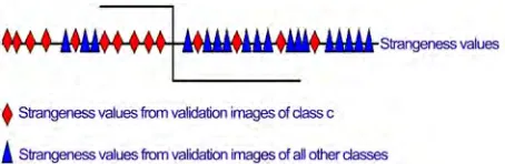
[image:7.595.310.537.77.151.2]

The strangeness is the thread to implement both rep-resentation and boosting (learning, inference, and predic-tion regarding classificapredic-tion). The strangeness, which implements the interface between the biometric representa-tion (including its attributes and/or parts) and boosting, combines the merits of filter and wrapper classification methods. The coefficients and thresholds for the weak learners, including the thresholds needed for open set recognition and rejection are learned using validation images, which are described in terms of components similar to those found during enrollment [21]. The best feature co- rrespondence for each component is sought between a validation and a training biometric image over the com-ponent (“parts” or “attributes”) defining that comcom-ponent. The strangeness of the best component found during training is computed for each validation biometric image under all its putative class labels c (c = 1,…,C). Assum-ing M validation biometric images from each class, one derives M positive strangeness values for each class c, and M(C – 1) negative strangeness values. The positive and negative strangeness values correspond to the case when the putative label of the validation and training image are the same or not, respectively. The strangeness values are ranked for all the components available, and the best weak learner hi is the one that maximizes the recognition rate over the whole set of validation biomet-ric images V for some component i and threshold θi. Boosting execution is equivalent to cascade classification [22]. A component is chosen as a weak learner on each

Figure 1. Learning Weak Learners (“Biometric Compone- nts”) as Stump Functions.

iteration (see Figure 1).

The level of significance α determines the scope for the null hypothesis H0. Different but specific alternatives can be used to minimize Type II error or equivalently to maximize the power (1 ─ β) of the weak learner [23]. During cascade learning each weak learner (“classifier”) is trained to achieve (minimum acceptable) hit rate h = (1

─ β) and (maximum acceptable) false alarm rate α (see Sect. 2) Upon completion, boosting yields the strong classifier H(x), which is a collection of discriminative bio-metric components playing the role of weak learners. The hit rate after T iterations is hTand the false alarm αT.

8. Score Normalization, Revision Theory,

and CMC Estimation

The practice of score normalization in biometrics aims at countering subject/client variability during verification. It is used (a) to draw sharper class or client boundaries for better authentication and (b) to make the similarity scores compatible and suitable for integration. The emp- hasis in this section is the former rather than the latter, which was already discussed in Section 7. Score normalization is concerned with adjusting both the client de-pendent scores and the thresholds needed for decision – making during post-processing. The context for score normalization includes clients S and impostors



S. One should not confuse post processing score normalization with normalization implemented during preprocessing, which is used to overcome the inherent variability in the image acquisition process. Such preprocessing type of normalization usually takes place by subtracting the mean (image) and dividing the result by the standard deviation. This leads to biometric data within the normalized range of [0, 1]. Score normalization during post-processing can be adaptive or empirical, and it requires access to additional biometric data prior and/or during the decision-making process.

The details for empirical score normalization and its effects are as follows [24]. Assume that the PDF of match (“similarity”) scores is available for both genuine transactions (for the same client), i.e., Pg, and impostor

transactions (between different clients), i.e., Pi. Such

(8)

enrollment or gained during the evaluation itself. One way to calculate the normalized similarity score ns for a match score m is to use Bayes’ rule

   

P P P P

ns g m  m g g m

where P(g) is the a priori probability of a genuine event and P(m│g) is the conditional probability of match score m for some genuine event g. The probability of m for all events, both genuine and impostor transactions, is

 

   



 



 

P m P g P_g m + 1 P g P_i m

The normalized score ns is then

   



 



 

P P_g P P_g 1 P P_i

ns g m _ g m   g m

The accuracy for the match similarity scores depends on the degree to which the genuine and impostor PDF approximate ground truth. Bayesian theory can determine optimal decision thresholds for verification only when the two (genuine and impostor) PDF are known. To com- pensate for such PDF estimation errors one should fit for the “overall shape” of the normalized score distribution, while at the same time seek to discount for “discrepanc- ies at low match scores due to outliers” [25]. The normalized score serves to convert the match score into a more reliable value.

The motivation behind empirical score normalization using evaluation data can be explained as follows. The evaluation data available during testing attempts to overcome the mismatch between the estimated and the real conditional probabilities referred to above. New (on – line) estimates are obtained for both Pg(m) and Pi(m), and the similarity scores are changed accordingly. As a result, the similarity score between a probe and its gallery cou- nterpart varies. Estimates for the genuine and impostor PDF, however, should still be obtained at enrollment time and/or during training rather than during testing. One of the innovations advanced by FRVT 2002 was the concept of virtual image sets. The availability of the similarity (between queries Q and targets T) matrix en-ables one to conduct different “virtual” experiments by choosing specific query P and gallery G sets as subsets of Q and T. Examples of virtual experiments include as- sessing the influence of demographics and/or elapsed time on face recognition performance. Performance scores relevant to a virtual experiment correspond to the P × G similarity scores. Empirical score normalization compr- omises, however, the very concept of virtual experiments. The explanation is quite simple. Empirical score normalization has no access to the information needed to de-fine the virtual experiment. As a result, the updated or normalized similarity scores depend now on additional information whose origin is outside the specific gallery and probe subsets.

Revision theory expands on score normalization in a principled way and furthers the scope and quality of biometric inference. Semi-supervised learning operates under the smoothness assumption (of supervised learning) that similar patterns should yield similar matching scores; and under the low-density separation assumption for both labeled and unlabeled examples. Training and testing are complementary to each other and one can revise both the labels and matching scores to better accommodate the smoothness assumption. Genuine and imposter individ-ual contributions, ranked using strangeness and p-values, are updated, if there is need to do so, in a fashion similar to that used during open set recognition. This contrasts with the holistic approach where matching scores are re-estimated using the Bayes rule and generative models as described earlier.

The basic tools for revision theory are those of pertur-bation, relearning, and stability to achieve better learning and predictions and therefore to make better inferences [26]. Perturbations to change labels and/or matching scores in regions of relatively high-density and then re-es-timate the margin together with quality measures for the putative assignments made, e.g., credibility and confide- ence (see Section 10). Gradient-descent and stochastic optimization are the methods of choice for choosing and implementing among perturbations using the regulariza-tion framework. Re-learning and stability are relevant as explained next. Transduction seeks consistent labels and matching scores for both training (labeled) and test (unlabeled) data. Poggio et al. [26] suggest it is the stability of the learning process that leads to good predictions. In particular, the stability property says that “when the training set is perturbed by deleting one example, the learned hypothesis does not change much. This stability property stipulates conditions on the learning map rather than on the hypothesis space.” Perturbations (“what if”) should therefore include relabeling, exemplar deletion (s), and updating matching scores. As a result of guided per-turbations more reliable and robust biometric inference and predictions become possible.

(9)

exactly one mate for each probe query, i.e., the gallery sets are singletons. Assume A classes enrolled in the gal-lery, N query example, the strangeness (“odds”) defined for k = 1 to yield (similar to cross TCM validation) NA values, A “valid”, and N(A-1) invalid (kind of imposters). Determine for each query and for their correct putative class assignment a, the corresponding p-value rank r ε (1, ..., A). The lower the rank r, the more typical the biometric sample is to its true class a. Tabulate the num-ber of queries for each class A and normalize by the total number of queries N. This yields an estimate for CMC. The presence of more than one mate for some or all of the probes in the gallery, e.g., Smart Gate and FRGC, which employ k > 1 and are thus more in tune with the strangeness and p-values definitions, can be handled in several ways. One way is to declare a probe matched at rank r if at least one of its mated gallery images shows up at that rank. Similar to the singleton case, tabulate the minimum among the p-values for all samples across their correct mates. Other possibilities would include retriev-ing all the mates or a fraction thereof at rank r or better and/or using a weighted metric that combines the simi-larity between the probe and its mates. There is also the possibility that the test probe set itself consists of several images and/or that both the gallery and the probe sets include several images for each subject. This can be dealt using the equivalent of the Hausdorff distance with the minimum over gallery sets performed in an iterative fashion for query sets or using the minimum over both the gallery and query sets pair wise distances. Last but not least, recall and precision (sensitivity and specificity) and F1 are additional (information retrieval) indexes that can be estimated using the strangeness and p-values in a fashion similar to CMC estimation.

9. Face Selection and Tracking

Face selection expands on the traditional role of face authentication. It assumes that multiple still image sets and/ or video sequences for each enrollee are available during training, and that a data streaming video sequence of face images, usually acquired from CCTV, becomes available during surveillance. The goal is to identify the subset of (CCTV) frames, if any, where each enrolled subject, if any, shows up. Subjects can appear and disappear as time progresses and the presence of any face is not necessarily continuous across (video) frames. Faces belonging to different subjects thus appear in a sporadic fashion across the video sequence. Some of the CCTV frames could ac- tually be void of any face, while other frames could include occluded or disguised faces from different subjects. Kernel k-means and/or spectral clustering [27] using biometric patches, parts, and strangeness and p-values for ty-

picality and ranking are proposed for face selection and tracking. This corresponds to the usual use of tracking during surveillance, while another use of tracking for identity management is deferred to the next section. Face selection counts as biometric inference. Biometric evidence accumulates and inferences on authentication can be made for familiar (“enrolled”) faces.

Spectral clustering is a recent methodology for segm- entation and clustering. The inspiration for spectral clustering comes from graph theory (minimum spanning trees (MST) and normalized cuts) and the spectral (eigen de-composition) of the adjacency/proximity (“similarity”) matrix and its subsequent projection to a lower dimen-sional space. This describes in a succinct fashion the graph induced by the set of biometric data samples (“pat-terns”). Minimizing the “cut” (over the set of edges con-necting k clusters) yields “pure” (homogeneous) clusters. Similar to decision trees, where information gain is re- placed by gain ratio to prevent spurious fragmentation, one substitutes the “normalized cut” (that minimizes the cut while keeping the size of the clusters large) for “cut.” To minimize the normal cut (for k = 2) is equivalent to minimize the Raleigh quotient of the normalized graph Laplace matrix L* where L* = D-1/2LD-1/2 with L = D – W; W is the proximity (“similarity”) matrix and the (di-agonal) degree matrix D is the “index” matrix that meas-ures the “significance” for each node. The Raleigh quo-tient (for k = 2) is minimized for the eigenvector z corre-sponding to the second smallest eigenvalue of L*. Given n data samples and the number of clusters expected k, spectral clustering (for k > 2) employs the Raleigh – Ritz theorem and leads among others to algorithms such as Ng, Jordan, and Weiss [28] where one (1) computes W, D, L, and L*; (2) derives the largest k eigenvectors zi

of L*; (3) forms the matrix UεRn × k by normalizing the row sums of zi to have norm 1; (4) cluster the samples

xi corresponding to zi using K-means.

An expanded framework that integrates graph-based semi-supervised learning and spectral clustering for the purpose of grouping and classification, i.e., label propa-gation, can be developed. One takes now advantage of both labeled and mostly unlabeled biometric patterns. The graphs reflect domain knowledge characteristics over nodes (and sets of nodes) to define their proximity (“similarity”) across links (“edges”). The solution pro-posed is built around label propagation and relaxation. The graph and the corresponding Laplacian, weight, and diagonal matrices L, W, and D are defined over both labeled and unlabeled biometric patterns. The harmonic function solution [29] finds (and iterates) on the (cluster) assignment for the unlabeled biometric patterns Yu as Y

= – (Luu)-1 Lul Yl with Luu the submatrix of L on

(10)

nodes. Each row of Yu reports on the posteriors for the

Cartesian product between k clusters and n biometric samples. Class proportions for the labeled patterns can be estimated and used to scale the posteriors for the unlabeled biometric patterns. The harmonic solution is in sync with a random (gradient) walk on the graph that makes predictions on the unlabeled biometric patterns according to the weighted average of their labeled neighbors.

An application of semi-supervised learning to person identification in low-quality webcam images is described by Balcan et al. [30]. Learning takes place over both (few) labeled and (mostly) unlabeled face images using spectral clustering and class mass normalization. The functionality involved is similar to face selection from CCTV. The graphs involved consists of i) time edges for adjacent frames likely to contain the same person (if moving at moderate speed); ii) color edges (over short time interval) assume person’s apparel the same; and iii) face edges for similarity over longer time spans. Label propagation and scalability become feasible using rank-ing [31] and semi-supervised learnrank-ing and parallel Map- Reduce [32] (in a fashion similar to Page Rank).

10. Identity Management

Identity management stands for another form of tracking. It involves monitoring the gallery of biometric templates in order to maintain an accurate and faithful rendition of enrolled subjects as times moves on. This facilitates re-liable and robust temporal mass screening and it repre-sents yet another for of biometric inference. The surveil-lance aspect is complementary and its role is to prevent imposters from subverting the security arrangements in place. Open set recognition [14], discussed earlier, is integral to surveillance but it does not provide the whole answer. The effective and efficient proper management of the gallery is the main challenge here and it is discussed next.

There are two main problems with identity management. One is to actively monitor the rendering of biometrics signatures and/or templates and the other is to upd- ate them if and when significant changes take place. The two problems correspond to active learning [12] and change detection [25], respectively. Active learning is con-cerned with choosing the most relevant examples needed to improve on classification both in terms of effective-ness (“accuracy”) and efficiency (“number of signatures needed”). The scope for active learning can be expanded to include additional aspects including but not limited to choosing the ways and means to accomplish effective-ness and efficiency, on one side, and adversarial learning, characteristic to imposters, on the other side. Our active learning solution [12] is driven by transduction and it is

built using strangeness and p-values. The p-values pro-vide a measure of diversity and disagreement in opinion regarding the true label of an unlabeled example when it is assigned all the possible labels. Let pi be the p-values obtained for a particular example xn + 1 using all possible

labels i = 1, . . . , M. Sort the sequence of p-values in descending order so that the first two p-values, say, pj and pk are the two highest p-values with labels j and k, respectively. The label assigned to the unknown example is j with a p-value of pj. This value defines the credibility of the classification. If pj (credibility) is not high enough, the prediction is rejected. The difference between the two p-values can be used as a confidence value on the predic-tion. Note that, the smaller the confidence, the larger the ambiguity regarding the proposed label. We consider three possible cases of p-values, pj and pk, assuming pj > pk: Case 1. pj high and pk low. Prediction “j” has high

credibility and high-confidence value; Case 2. pj high and pk high. Prediction “j” has high credibility but low-confidence value; Case 3. pj low and pk low.

Predic-tion “j” has low credibility and low-confidence value. High uncertainty in prediction occurs for both Case 2 and Case 3. Note that uncertainty of prediction occurs when pj≈ pk. Define “closeness” as I (xn + 1) = pj - pk to indicate the quality of information possessed by the example. As I (xn + 1) approaches 0, the more uncertain we are about

classifying the example, and the larger the margin infor-mation gain from “advise” is. Active learning will add this example, with its true label, to the training set because it provides new information about the structure of the biometric data model. Extensions to the active learning inference strategy describe above will incorporate error analysis and population diversity characteristic of pattern specific error inhomogeneities (PSEI) [14].

The basics for change detection using martingale are as follows [33]. Assume time-varying multi-dimensional data (stream) matrix R = {R(j) = xj} where R(j) are “columns” and stand for time-varying (data stream) biometric vectors. Assume that seeding provides some initial R(j) with j = 1, …, 10. K-means clustering will find (in an iterative fashion) center “prototypes” Q(k) for the data stream (seen so far). Define the strangeness correspond-ing to R(j) using the cluster model (with R = {xj} stand-ing for data stream and c standing for cluster center) and the Euclidean distance d(j) between R(j) and Q(k) for j > = 10 and k = j – 9 as



R, j



j s x  x c

Define p-values as





















1, y ,1 , , y ,

# : # :

i i i i

j i i j i

p

j s s j s s



 i

 

_    _

x  x

(11)

2, …, I and θi is randomly chosen from [0, 1] at instance i. Define a family of martingale starting with Mε(0) = 1 and continuing with Mε(j) indexed by ε in [0, 1]

 



 

1



1

M j

i i

j p 

 _ 





The martingale test

 

0M j 

rejects the null hypothesis H0 “no change in the data stream” for H1 (“change detected in data stream”) when M (j) > = λ with the value for λ (empirically chosen to be greater than 2) determined by the FAR one is willing to accept, i.e., 1/λ = FAR. An alternative (parametric) test, e.g., SPRT, will employ the likelihood ratio (LR) with B < LR < A and decide for H0 as soon as LR(j) < B, decide for the alternative H1 (“change”) when LR(j) > A, with B ≈β (1 – α) and A ≈ (1 – β)/α using αfor test signifi-cance (“size”) and (1 – β) for test power. The changes (“spikes”) found can identify critical (transition) states, e.g., ageing, and model an appropriate Hidden Markov Model (HMM) for personal authentication and ID man-agement.

11. Conclusions

This paper proposes a novel all encompassing method-ology for robust biometric inference and prediction built around randomness and complexity concepts. The methodology proposed can be mapped to other types of in-formation beyond the biometric modality discussed here. The theoretical framework advanced here for biometric information management is model-free and non-parametric. It draws support from discriminative methods using likelihood ratios to link the Bayesian framework, statis-tical learning theory (SLT), and Information Theory (IT) using transduction, semi-supervised learning, and mutual information between biometric signatures and/or tem-plates and their labels. Several topics on biometric infer-ence related to i) multi-level and multi-layer data fusion including quality and multi-modal biometrics; ii) cross- matching of capture devices, revision theory, and score normalization; iii) face selection and tracking; and iv) identity management and surveillance were addressed using an integrated approach that includes transduction and boosting for ranking and sequential fusion/aggregation, respectively, on one side, and active learning and change /outlier/intrusion detection using information gain and martingale, respectively, on the other side.

One venue for future research would expand the scope of biometric space regarding information contents and processes. Regarding the biometric space, Balas and Si- nha [34] have argued that “it may be useful to also employ region-based strategies that can compare noncontig-

uous image regions.” They further show that “under cer-tain circumstances, comparisons [using dissociated dip- ole operators] between spatially disjoint image regions are, on average, more valuable for recognition than fea-tures that measure local contrast.” This is consistent with the expectation that recognition-by-parts architectures [21] should learn [using boosting and transduction] “op-timal” sets of regions’ comparisons for biometric authen-tication across varying data capture conditions and con-texts. The choices made on such combinations for both multi-level and multi-layer fusion amount to “rewiring” operators and processes. Rewiring corresponds to an additional processing and competitive biometric stage. As a result, the repertoire of information available to biomet-ric inference will now range over local, global, and non- local (disjoint) data characteristics with an added tempo-ral dimension. Ordinal rather than absolute codes are feasible in order to gain invariance to small changes in inter-region and temporal contrast. Disjoint and “rewired” patches of information contain more diagnostic information and are expected to perform best for “expres-sion”, self-occlusion, and varying image capture conditions. The multi-feature and rewired based biometric im-age representations and processes together with exemplar-based biometric representations enable flexible matching. The added temporal dimension is characteristic of video sequences and it should lead to enhanced biometric authentication and inference performance using set simi-larity. Cross-matching biometric devices is yet another endeavor that could be approached using score normali-zation, non-linear mappings, and revision theory (see Section 8).

Another long-term and needed research venue should consider useful linkages between information theory, the Bayesian framework, and statistical learning theory to advance modes of reliable and robust reasoning and in-ference with directed application to biometric inin-ference. Such an endeavor will be built around the regularization framework using fidelity of representation, compressive sensing, constraints satisfaction and optimization subject to penalties, and margin for prediction. Biometric dicti- onaries are also needed for biometric processes to choose from for flexible exemplar-based representation, reason-ing, and inference, and to synthesize large-scale datab- ases for biometric evaluations. The ultimate goal is to develop powerful and wide scope biometric language(s) and the corresponding biometric reasoning (“inference”) apparatus in a fashion similar to the way language and thought are available for human (“practical”) intelligence and inference [35].

12. References

(12)

and P. Sturges Eds., International Encyclopedia of Information and Library Science, Routledge, London, 2003, pp. 263-278.

[2] N. Schmid and H. Wechsler, “Information Theoretical (IT) and Statistical Learning Theory (SLT) Characteriza-tions of Biometric Recognition Systems,” SPIE Elec-tronic Imaging: Media Forensics and Security, San Jose, CA, Vol. 7541, 2010, pp. 75410M-75410M-13.

[3] N. Poh, T. Bourlai, J. Kittler et al., “Benchmark Qual-ity-Dependent and Cost-Sensitive Score-Level Multimo-dal Biometric Fusion Algorithms,” The IEEE Transaction on Information Forensics and Security, Vol. 4, No. 4, 2009, pp. 849-866.

[4] N. Poh, T. Bourlai and J. Kittler, “A Multimodal Biomet-ric Test Bed for Quality-dependent, Cost-Sensitive and Client-Specific Score-Level Fusion Algorithms,” Pattern Recognition, Vol. 43, No. 3, 2010, pp. 1094-1105.

[5] H. B. Barlow, “Unsupervised Learning,” Neural Compu-tation, Vol. 1, 1989, pp. 295-311.

[6] Y. D. Rubinstein and T. Hastie, “Discriminative Versus Informative Learning,” Knowledge and Data Discovery (KDD), 1997, pp. 49-53.

[7] J. Gonzalez-Rodriguez, P. Rose, D. Ramos, D. T. Tole-dano and J. Ortega-Garcia, “Emulating DNA: Rigorous Quantification of Evidential Weight in Transparent and Testable Forensic Speaker Recognition,” IEEE Transac-tion on Audio, Speech and Language Processing, Vol. 15, No. 7, 2007, pp. 2104-2115.

[8] C. Champed and D. Meuwly, “The Inference of Identity in Forensic Speaker Recognition,” Speech Communication, Vol. 31, No. 2-3, 2000, pp. 193-203.

[9] D. Dessimoz and C. Champod, “Linkages between Bio-metrics and Forensic Science,” in A. K. Jain, Ed., Hand-book of Biometrics, Springer, New York, 2008.

[10] B. Black, F. J. Ayala and C. Saffran-Brinks, “Science and the Law in the Wake of Daubert: A New Search for Sci-entific Knowledge,” Texas Law Review, Vol. 72, No. 4, 1994, pp. 715-761.

[11] M. Li and P. Vitanyi, “An Introduction to Kolmogorov Complexity and Its Applications,” 2nd Edition, Springer- Verlag, Germany, 1997.

[12] S. S. Ho and H. Wechsler, “Query by Transduction,” IEEE Transaction on Pattern Analysis and Machine In-telligence, Vol. 30, No. 9, 2008, pp. 1557-1571.

[13] T. Melluish, C. Saunders, A. Gammerman, and V. Vovk, “The Typicalness Framework: A Comparison with the Bayesian Approach,” TR-CS, Royal Holloway College, University of London, 2001.

[14] F. Li and H. Wechsler, “Open Set Face Recognition Us-ing Transduction,” IEEE Transaction on Pattern Analysis and Machine Intelligence, Vol. 27, No. 11, 2005, pp. 1686- 1698.

[15] V. Vapnik, “Statistical Learning Theory,”Springer, New York, 1998.

[16] O. Chapelle, B. Scholkopf and A. Zien (Eds.), “Semi- Supervised Learning,” MIT Press, USA, 2006.

[17] T. M. Cover and P. Hart, “Nearest Neighbor Pattern Classification,” IEEE Transaction on Information Theory, Vol. IT-13, 1967, pp. 21-27.

[18] Y. Freund and R. E. Shapire, “Experiments with a New Boosting Algorithm,” Proceedings of 13th International Conference on Machine Learning (ICML), Bari, Italy, 1996, pp. 148-156.

[19] F. H. Friedman, T. Hastie and R. Tibshirani, “Additive Logistic Regression: A Statistical View of Boosting,” Annals of Statistics, Vol. 28, 2000, pp. 337-407.

[20] V. Vapnik, “The Nature of Statistical Learning Theory” 2nd Edition, Springer, New York, 2000.

[21] F. Li and H. Wechsler, “Face Authentication Using Rec-ognition-by-Parts, Boosting and Transduction,” Interna- tional Journal of Artificial Intelligence and Pattern Rec-ognition (IJPRAI ), Vol. 23, No. 3, 2009, pp. 545-573.

[22] P. Viola and M. Jones, “Rapid Object Detection Using a Boosted Cascade of Simple Features,” Proceedings of the Computer Vision and Pattern Recognition Conference (CVPR), Kauai, Hawaii, 2001, pp. I-511-I-518.

[23] R. O. Duda, P. E. Hart and D. G. Sork, “Pattern Classifi-cation,” 2nd Edition, Wiley, New York, 2000.

[24] A. Adler, “Sample Images Can be Independently Regen-erated from Face Recognition Templates,” 2003. http://www.site.uotawa.ca/~adler/publications/2003/adler -2003-fr-templates.pdf.

[25] T. Poggio and S. Smale, “The Mathematics of Learning: Dealing with Data” Notices of American Mathematical Socity, Vol. 50, No. 5, 2003, pp. 537-544.

[26] T. Poggio, R. Rifkin, S. Mukherjee and P. Niyogi, “Gen-eral Conditions for Predictivity of Learning Theory,” Nature, Vol. 428, No. 6981, 2004, pp. 419-422.

[27] I. S. Dhillon, Y. Guan and B. Kulis, “Kernel k-means, Spectral Clustering and Normalized Cuts,” Proceedings of the Conference on Knowledge and Data Discovery (KDD), Seattle, WA, 2004.

[28] A. Y. Ng, M. I. Jordan and Y. Weiss, “On Spectral Clus-tering: Analysis and an Algorithm,” Neural Information Processing Systems (NIPS) 14, MIT Press, Boston, MA, 2002, pp. 849-856.

[29] X. Zhu, Z. Ghahramani and L. Lafferty, “Semi-Supervised Learning Using Gaussian Fields and Harmonic Func-tions,” Proceedings of the 20th International Conference on Machine Learning (ICML), Washington, DC, 2003, pp. 912-919.

[30] M. F. Balcan, A. Blum, P. P. Choi, J. Lafferty, B. Pan-tano, M. R. Rwebangira and X. Zhu, “Person Identifica-tion in Webcam Images: An ApplicaIdentifica-tion of Semi-Supervised Learning,” Proceedings of 22nd ICML Workshop on Learning with Partially Classified Training Data, Bonn, Germany, 2005, pp. 1-9.

[31] K. Duh and K. Kirchhoff, “Learning to Rank with Par-tially Labeled-Data,” SIGIR, Singapore, 2008, pp. 20-27.

(13)

Methods for Natural Language Processing (ACL-IJCNLP), Singapore, 2009, pp. 58-65.

[33] S. S. Ho and H. Wechsler, “A Martingale Framework for Detecting Changes in the Data Generating Model in Data Streams,” IEEE Transaction on Pattern Analysis and Machine Intelligence, No. 99,2010 (to appear).

[34] B. J. Balas and P. Sinha, “Region-Based Representations for Face Recognition,” ACM Transactions on Applied Perception, Vol.3, No. 4, 2006, pp. 354-375.