Munich Personal RePEc Archive
Deconstructing Job Search Behavior
Banfi, Stefano and Choi, Sekyu and Villena-Roldán,
Benjamin
Chilean Ministry of Energy, University of Bristol, University of Chile
25 January 2019
Deconstructing Job Search Behavior
∗Stefano Banfi
Ministry of Energy, Chile
Sekyu Choi
University of Bristol
Benjam´ın Villena-Rold´an
CEA, DII, University of Chile
January 25, 2019
Abstract
We use an unusually rich data from a Chilean job board to document novel facts regarding job search for unemployed and employed seekers. We show how application behavior is influenced by (1) demographics such as gender, age, and marital status, (2) alignment between applicant wage expectations and wage offers, (3) applicant fit into ad requirements such as education, experience, job location and occupation (4) timing variables, including unemployment duration, job tenure (for on-the-job searchers) and business cycle conditions. This empirical evidence can discipline current and future search-theoretical frameworks.
Keywords: Online job search, Applications, Search frictions, Unemployment, On-the-job search,
Networks. JEL Codes: E24, J40, J64
∗Email: [email protected], [email protected] and [email protected]. We thank Guido Menzio,
Brenda Samaniego de la Parra, Jan Eeckhout, Shouyong Shi, Yongsung Chang, Francois Langot, Bari¸s Kaymak, and seminar participants at Cardiff University, University of Manchester, Diego Portales University, the 2016 Midwest Macro Meetings, the 2016 LACEA-LAMES Workshop in Macroeconomic, the Search & Matching workshop at the University of Chile, 2017 SAM Meetings in Barcelona, Spain, 2017 SECHI Meeting, 2017 SM3 Workshop, and Univer-sidad de Los Andes Bogot´a, Universit´e de Montr´eal, Universidad de Chile, and the IDSC of IZA Workshop: Matching Workers and Jobs Online for insightful discussion and comments. Villena-Rold´an thanks for financial support the FONDECYT projects 1151479 and 1191888, and the Institute for Research in Market Imperfections and Public Pol-icy, ICM IS130002, Ministerio de Economa, Fomento y Turismo de Chile. We are indebted towww.trabajando.com
Introduction
What kind of jobs workers look for and how much effort they exert are critical for labor market
outcomes. Job search determines wages and job allocations in the economy to a large extent. As applications are tentative allocations, they are of prime importance to understand ex post outcomes such as the unemployment rate, mobility, efficiency, and income inequality. Thus, we use
data from the job posting website www.trabajando.comto deconstruct behavior into two margins and quantify their impact on application decisions: First, an intensive margin, where we focus
on independent characteristics of applicants or job postings, as studied in Faberman and Kudlyak
(forthcoming); Gomme and Lkhagvasuren(2015);Leyva (2018);Mukoyama, Patterson, and S¸ahin
(2018). Second, a selective margin, where the focus is on coincidences between characteristics of the worker and the job. To the best of our knowledge, we are the first to systematically study both margins jointly, providing a comprehensive catalogue of search behavior under a wide array
of circumstances.
We use thenetwork formed by job seekers linked through common job applications to construct
the choice set of an applicant as the list of all ads applied by seekers linked with her. Our methodol-ogy overcomes the problem of only observing actual choices in the data, a recurrent problem when
studying consumption choices in industrial organization and marketing, as inVan Nierop, Bronnen-berg, Paap, Wedel, and Franses(2010) and Abaluck and Adams(2017), among others. It also has two important advantages over alternatives in the literature:1
First, it relies on applicant revealed
preferences over a probably large number of observable and unobservable (to the econometrician) job characteristics to define similarities among jobs, instead of often few arbitrary dimensions such
as locations, occupations, or industry. Using arbitrary choice sets, one would inevitably ignore attempted mobility across segments, a likely important issue as shown inCarrillo-Tudela and Viss-chers (2014). Second, the network approach allows us to define individual choice sets, generating
key variability for parameter identification.
With respect to theintensive margin, our empirical exercise reveals the effects of different traits
on the probability of applying to a job ad. Unconditionally, in our sample females apply more tan males, but once we control for ad and worker characteristics, the result reverses. This suggests that
males apply to a wider range of job positions, other things equal. Marital status matters: employed married males apply more than their single counterparts, and females have the reverse pattern. We also document that the application probability increases with age for the unemployed, but for the
employed, age seems of little relevance. Although the job finding probability declines in age (Choi, Janiak, and Villena-Rold´an,2015;Menzio, Telyukova, and Visschers,2016), both findings may be
consistent as long as older jobseekers react to scarcer job opportunities and higher opportunity cost
1
We could have defined choice sets as segments defined by an arbitrary set of job characteristics asS¸ahin, Song, Topa, and Violante(2014) andHerz and van Rens(2015), or by clustering algorithms asBanfi and Villena-Rold´an
of time.
We find evidence of stock-flow matching behavior:2
new job seekers in the website (the flow) apply to the stock of job adverts during their initial time on the platform. When time passes, the inflow of job seekers becomes part of the stock of individuals, who then try to match with the
new flow of job positions. Gregg and Petrongolo(2005) andColes and Petrongolo (2008) provide evidence for stock-flow matching in different contexts. In our analysis, we show that unemployed
individuals apply more for newer job ads, other things equal, which is consistent with distaste for “phantom” job postings.3
However, we observe the opposite effect for on-the-job seekers. On top
of this, we show that workers apply more to job postings advertising more vacancies, suggesting that individuals respond to indications of the likelihood of receiving an offer given an application. We also find a decreasing probability of application as the unemployed search duration increases,
an important issue for the design of unemployment insurance policies as stated by Faberman and Kudlyak (forthcoming). For on the job seekers, we find that the average application probability
seems flat with respect to tenure in the current job. This is qualitatively consistent with the evidence of job-to-job flows inMenzio, Telyukova, and Visschers(2016). This finding is relevant to discipline models explaining job-to-job transitions and frictional wage dispersion as in Hornstein,
Krusell, and Violante(2011).
The intensive margin shows a very large variability over the business cycle, but also a nuanced
cyclical behavior. For on-the-job seekers, it is procyclical; for the unemployed, it is procyclical almost always, but countercyclical for high unemployment rates. A non-monotonic response of job
search effort to cyclical conditions may help explain disparate findings in the literature.4
As for theselective margin, we find that applicants show misalignment distaste in general: they are highly sensitive to the fit between worker traits and ad requirements in terms of educational
level, experience, location, wages, and occupation. This distaste is apparent in terms of location, i.e. the probability of application decreases in the geographical distance between worker and employer,
and in terms of occupation. The results are nuanced for other dimensions: job seekers target a most preferred type of job on average, but it is not necessarily the one that perfectly matches their
current characteristics. For instance, all workers, especially the employed, possess more experience than the minimum required by ads on average.
In the evidence we read that employed job seekers are more daring or ambitious: their
proba-bility of application peaks when they are slightly underqualified in terms of education and apply more to jobs with wages above their expectations on average. In contrast, the unemployed apply
the most to jobs that have the same educational requirements that they posses and apply more
2
SeeTaylor(1995),Coles and Muthoo(1998),Coles and Smith(1998) andEbrahimy and Shimer(2010), among others.
3
SeeAlbrecht, Decreuse, and Vroman(2017);Ch´eron and Decreuse(2016). 4
to ads matching their own wage expectations. Thus, the evidence points to unemployed seekers
maximizing job offer chances, while employed ones try to climb the job ladder.
We provide further evidence regarding the interaction between misalignment distaste and three time domains: life cycle, employment status duration, and business cycles. Our findings show
that age, depending on employment status, attenuate or intensify the compliance of job seekers to ad requirements. The oldest jobseekers become more insensitive to educational requirements
if employed, while the younger unemployed group seems less attracted to jobs for which they are overqualified. All workers seem to concern less about experience required as they age, especially
if unemployed. Employed workers are substantially more open to move to a distant location for a job as they age. Young jobseekers are more ambitious than their older counterparts: if employed they aim for wages higher than their expectations; if unemployed, they are less sensitive to the
offered-expected wage gap. Occupation misalignment decreases in age and is always greater for the unemployed.
Workers change their application decisions according to their tenure in a nuanced way. On one hand, the employed are more ambitious if they have a tenure below the median: they apply slightly more to ads for which they are underqualified in education, and exhibit a slight
misalign-ment distaste in experience (while long-tenured workers do not care about this). On the other hand, long-tenured workers are moreflexible: the distaste for worker-job distance and occupational
misalignment decays in tenure. This suggests that geographical and occupational mobility involve seasoned job movers. In addition, the wage misalignment sensitivity is roughly constant over tenure
levels.
For unemployed seekers, as their search spell increases, they become more conservative: they apply more to job ads offering lower wages and requiring lower education. They become more
flexible, too: they exhibit lower sensitivity to experience requirements and lower distaste for occu-pational misalignment . However, the distaste for geographical distance increases in unemployment
duration.
The variation of the selective margin over the business cycle is small in comparison to the
intensive margin variation. The unemployed reduce their distaste for jobs for which they are overqualified in education. Middle-tenured employed workers and long-term unemployed seekers become slightly more sensitive to experience misalignment . On-the-job seekers dislike less distant
and low wage jobs when the unemployment rate is at its highest. The occupational distaste seems countercyclical, except for the highest quartile of unemployment rates.
We finally explore whether gender affects the selective margin. Males seem eager to take more risks in some dimensions. They apply more often to jobs with lower education requirements if employed, and jobs with higher education requirements if unemployed. Females consistently comply
less distant jobs. Employed males also seem more open to occupational moves.
Our paper is related to a growing literature which use data from online job-posting/search websites in order to study different aspects of frictional markets. Kudlyak, Lkhagvasuren, and Sysuyev (2013) study how job seekers direct their applications over the span of a job search.They
find some evidence on positive sorting of job seekers to job postings based on education and how this sorting worsens the longer the job seeker spends looking for a job (the individual starts
ap-plying for worse matches). Faberman and Kudlyak (forthcoming) use online job board data to study the intensive margin of job search. Marinescu and Rathelot (2015) use information from
www.careerbuilder.com and find that job seekers are less likely to apply to jobs that are farther
away geographically. Marinescu and Wolthoff(2015) use the same job posting website to study the relationship between job titles and wages posted on job advertisements. They show that job titles
explain nearly 90% of the variance of explicit wages. Banfi and Villena-Rold´an (forthcoming) and
Banfi, Choi, and Villena-Rold´an (2018) use data from this website to find substantial evidence of
directed search and assorative matching, providing complementary evidence related to the selective margin.
The data
We use data fromwww.trabajando.com(henceforth the website) a job search engine with presence in mostly Spanish speaking countries: as of September of 2017, the list comprises Argentina, Brazil,
Colombia, Chile, Mexico, Peru, Portugal, Puerto Rico, Spain, Uruguay and Venezuela. Our data covers a sample of job postings and job seekers in the Chilean labor market, between January 1st 2008 and December 24th, 2016. The raw information in the dataset contains more than 14 million
single applications, from around 1.5 million job seekers, to around 270 thousand job ads.
Our dataset has detailed information on both applicants and recruiters. First, we observe entire
histories of applications from job seekers and dates of ad postings (and repostings) for recruiters. Second, we have detailed information for both sides of the market. For job seekers we observe date of birth, gender, nationality, place of residency (”comuna” and ”regi´on”, akin to county and US
state, respectively), marital status, years of experience, years of education, college major and name of the granting institution of the major.5
We have codes for occupational area of the current/last
job of individuals,6
information on their salary and both their starting and ending dates.
In terms of the website’s platform, job seekers can use the site for free, while firms are charged
for posting ads. Job advertisements are posted for a minimum of 60 days, but firms can pay additional fees to extend this term.7
5
This information is for any individual with some post high school education. 6
We observe a one-digit classification, created by the website administrators. 7
For each posting, we observe its required level of experience (in years), required college major (if
applicable), indicators on required skills (specific, computing knowledge and/or “other”) how many positions must be filled, the same occupational code applied to workers, geographic information (“regi´on” only) and some limited information on the firm offering the job: its size (number of
employees in brackets) and industry (1 digit code). Educational categories are primary (one to eight years of schooling),high school (completed high school diploma, 12 years), technical tertiary
education (professional training after high school, usually 2-4 years),college (completed university degree, usually 5-6 years) and post-graduate (any schooling higher than college degree).
A novel feature of the dataset, compared to the rest of the literature, is that the website asks job seekers to record their expected salary, which they can then choose to show or hide from prospective employers. Recruiters are also asked to record the expected pay for the job posting, and given the
same choice whether to make this information visible or not to the applicants. Naturally, one could question the reliability of wage information which will be ultimately hidden from the other side of
the market. Banfi and Villena-Rold´an (forthcoming) address the potential issue of “nonsensical” wage information in job ads by comparing the sample of explicit vs. implicit (job ads without any salary information) postings by firms, and find that observable characteristics predict fairly well
implicit wages and vice versa. Moreover, even if employers choose to hide wage offers, they are used in filters of the website for applicant search. Hence, employers are likely to report accurately even
if their wage offers are not shown because misreporting may generate adverse consequences. On the other hand, a major caveat of our dataset is the absence of information on activities performed
outside the website: individuals seeking for jobs through other means, and more importantly, outcomes of job applications.
For the remainder of the paper, we restrict our sample to consider only individuals working
under full-time contracts and those unemployed. We further restrict our sample to individuals aged 23 to 60. We discard individuals reporting desired net wages above 5 million pesos.8
This
amounts to approximately 8,347 USD per month9
, which is higher than the 99th percentile of the Chilean wage distribution, according to the 2013 CASEN survey.10
We also discard individuals
who desire net wages below 159 thousand pesos (around 350 USD) a month (the legal minimum wage at the start of our considered sample). Consequently, we also restrict job postings to those offering monthly salaries within those bounds.
Our unit of analysis are individualapplications. We restrict our sample to individuals who were
8
In the Chilean labor market wages are usually expressed in a monthly rate net of taxes, and mandatory contribu-tions to health (7% of monthly wage), to fully-funded private pension system (10%), to disability insurance (1.2%), and mandatory contribution to unemployment accounts(0.6%)
9
Using the average nominal exchanges rate between 2013-16,https://si3.bcentral.cl/Siete/secure/cuadros/ home.aspx.
10
actively looking for a job (i.e., made an application) and job postings that received at least one
application. While we observe long histories of job search for a significant fraction of workers (some workers have used the website for several years), we consider only applications pertaining to their last job search “spell”, which we define as the time window between the last modification/creation of
their online curriculum vitae (cv) in the website and the time of their last submitted application or the one year mark, whichever happens first. Since individuals maintain information about their last
job in their online profile, as well as contact information and salary expectations, we assume that any modification of this information is done primarily when individuals who are currently working
or who have already used the website in the past are ready to search in the labor market again. We cannot infer any labor transition based on application behavior because employed individuals may keep searching for jobs, and unemployed individuals may search outside of the website. We
further drop individuals who apply to more than the 99-th percentile of job applicants in terms of number of submitted applications in the defined window.
Table 1 shows descriptive statistics for the job searchers in our sample. From the table we observe that the average age is 33.5 and that job seekers are comprised of mostly single males, with 59.71% being unemployed (86,687 unemployed seekers from a total of 215,169 individuals.).
Average experience hovers around eight years. Job seekers in our sample are more educated than the average in Chile, with 41.84% of them having a college degree, compared to 25% for the rest
of the country in the comparable age group (30 to 44 years of age), according to the 2013 CASEN survey. There is also a big discrepancy by labor force status: unemployed seekers are significantly
less educated in the website.
From the table we can also observe that most job seekers claim occupations related to man-agement (around 20%) and technology (around 25%) and that average expected wages are
ap-proximately (in thousands) CLP$ 1,087 and CLP$ 592 for employed and unemployed seekers, respectively. For comparison, the 2013-16 average minimum monthly salary in Chile was around
CLP $ 226 thousand.11
In terms of search activity, the average search spell amounts to around five weeks. The amount
of time searching for a job is higher for those employed than for the unemployed: 5.24 versus 4.83 weeks respectively. In terms of applications, both groups show very similar choices, with around 1.52 submitted applications.
Application probabilities and job seeker preferences
In this section, we analyze empirically which attributes of heterogeneous jobs attract more appli-cations from heterogeneous job seekers. To do this, we first need to determine which is the relevant
11
Table 1: Characteristics of Job Seekers
Employed Unemployed Total
Demographics
Age 33.77 33.25 33.46
Males 0.62 0.54 0.57
Married 0.34 0.28 0.30
Experience (years) 8.28 7.64 7.90
Wages (thousand CLP) 1,087 592 792
Tenure (weeks) 177.96 – 177.96
Unemployment duration (weeks) – 60.20 60.20
Education level (%)
Primary (1-8 years) 0.12 0.25 0.2
High School 17.94 36.89 29.25
Technical Tertiary 26.56 28.82 27.91
College 54.22 33.48 41.84
Post-graduate 1.17 0.55 0.8
Occupation (%)
Management 23.5 17.85 20.12
Technology 31.59 21.21 25.39
Not declared 20.29 42.54 33.57
Rest 24.62 18.4 20.92
Search Activity
weeks searching on website 5.24 4.83 4.99
Number of applications 1.49 1.53 1.52
Observations 86,687 128,482 215,169
set of job ads for each individual in our sample. However, our dataset only contains information on actual applications and no information is collected by the website on total number of searches nor
clicks on job postings by individuals. Thus, we do not have sample variation in terms of job ads: we only observe those that individuals choose to apply to, but not those which are observed but
then discarded by seekers. This problem of “consideration sets” (i.e. the set of products consumers are aware of) is addressed in the literature in marketing and industrial organization (Van Nierop, Bronnenberg, Paap, Wedel, and Franses, 2010; Abaluck and Adams, 2017), but our approach is
essentially different. Nevertheless, we hypothesize that our network-revealed preference approach could be used in this literature, provided databases identify purchased goods by each consumer.
Market segmentation through network analysis.
We could consider the cross between all job seekers and all job ads that are time feasible in our
ads for her to screen and choose, implying an unrealistic effort for workers. Second, since we truly
try to characterize an actual decision-making process, by introducing job ads never considered by the applicant in her choice set, there is a sample selection as we include extraneous observations into the sample. Third, a more practical issue is that the size of the estimating sample becomes
simply too large to handle,12
making the task of even simple calculations infeasible.
We could create choice sets by using clustering of job ads using their traits as in Banfi and
Villena-Rold´an(forthcoming). However, such an approach links workers to a fixed set of ads, with little or null cross-sectional variation across similar applicants. Instead, our approach uses revealed
preferences of workers to construct individual consideration or choice sets based on coincidental choices made by other applicants. In reality, workers potentially apply to jobs considering a large number of potential characteristics, many of which we can observe. The revealed preference
ap-proach circumvents the problem of defining what the relevant information is for workers. We only determine the relevant set of ads for each worker based on their actual choices, regardless of the
way they process their information.
To formalize this notion, we use the network formed by job seekers to determine which job postings are relevant to them. Assume that each individual represents a node in the network, and
that a link between nodes is defined ashaving applied to the same job posting. For each job seeker
w, we define the set of relevant job postings A1
w as the union of all job postings applied by the
set of all job seekers linked to w. This is what we define as a network of degree 1, since for each individual, we only consider their immediate links (1 degree of separation).
Following this logic, the network of degree 0 is the original dataset for individual w(A0
w), since
the network contains only information of job seekers and their applications (no information on links is used). On the other hand, a network of degree 2 is defined as the network which considers both
job seekers linked directly tow, in addition to those who are linked with the links ofw(job seekers have 2 degrees of separation), giving rise to the setA2
w. We can continue with this logic iteratively,
until forming the set A∞
w, which is the cross between each job seeker w and all job postings aas long as they are connected somehow through the network.13
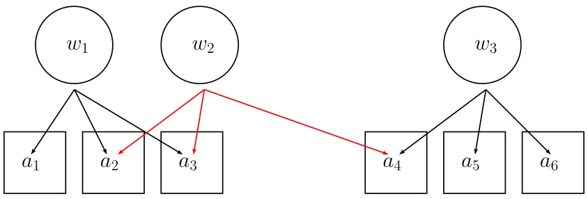
Figure 1 shows an example of the network algorithm and the resulting datasets. In the figure there are three workers, {w1, w2, w3} and six job postings, {a1, a2, a3, a4, a5, a6}. Consider worker
w1. She has applied to three jobs, thusA0w1 ={a1, a2, a3}and is linked tow2 through applications
to{a2, a3}. Sincew2 also applied to job positiona4, one can infer that some characteristic ofa4 is
not desirable tow1. If we consider networks of degree 1,a4 would be included in the set of relevant
ads for the first worker. Notice also that in this example, w1 is not directly linked with w3, or in
12
With our sample constraints we have 215,000 workers who could potentially apply to 20,000 job ads when they change their CV, a very conservative lower bound if they stay actively applying for several weeks. Thus, the exploded set contains 215,000×20,000 = 4,3 billions of potential applications.
13
Technically, the setA∞w and the exploded dataset differ if there are isolated pairs or groups of individuals who
w
1w
2w
3 [image:11.612.81.503.70.213.2]a
1a
2a
3a
4a
5a
6Figure 1: Example of a network formed by workers {w1, w2, w3}. Worker w1 is linked to worker w2 by common applications to adsa2anda3 but is not linked withw3 in the network of degree 1. All workers are linked in the network of degree 2.
our language, the degree of separation between these two workers is higher than 1. Again, considering the first worker, we have A0
w1 = {w1, w2, w3}, and as discussed above,
A1
w1 ={a1, a2, a3, a4}. Given thatw1 and w2 are linked and thatw2 is linked withw3, the relevant
job ads forw1, given a network of degree 2, isA 2
w1 ={a1, a2, a3, a4, a5, a6}. In our simple example,
the network of degree 2 is already the “exploded” network (all ads to all workers). The formal definition of a one-degree-of-separation ad set for a workerw is
A1
w =
[
v:A0w∩A0v6=∅
A0
w∪ A
0
v
which can be generalized for other degrees of separation.14
In what follows, we will concentrate on networks of degree one only.
In table 2, we present information on the resulting number of relevant job postings per worker and workers per job posting, given a network of degrees one. The median number of relevant
job postings (a) is 16 postings per job seeker, with employed seekers being related to more posts (19) than those unemployed (16). The number of potential ads exhibits quite the amount of variation, going from 2 (tenth percentile of distribution) to 104 and 89 for unemployed and employed
respectively (ninetieth percentile). Given the sets of related job ads, mean application rates,15
are 22.3% for the entire sample, with unemployed seekers applying to 23.2%, while employed ones do
14
The generalization follows a recursive definition
As w=
[
v:As−1
w ∩A
0
v6=∅ As−1
w ∪ A
0
v
which depends onA0
w and the definition ofA
1
w.
15
Defined as the number of effective applications to total ads for workerw:
|A0
w|
|A1
Table 2: Number of relevant ads (a) per worker (w) Potential ads for a worker
All U E
percentile 10 2 2 2
percentile 50 16 16 19
percentile 90 96 104 87
mean 38.5 40.7 36.8
standard deviation 68.1 73.8 57.1
mean applications (%) 22.3 23.2 20.9
Notes: The table shows the number of relevant job postings per job seeker given a network of degree 1 (see main text). Statistics separated by labor force status of job seeker (U = unemployed, E = employed). Standard errors in parentheses. One, two, and three asterisks indicate significance at 10%,5%, and 1%, respectively.
so for 20.9% of their relevant ads.
Although our network approach allows us to build choice sets for applicants, it is unlikely that all the ads in the set are equally considered.16
In any given network induced set of choices for each workerw, there is heterogeneity in the relevance of job ads, according to how strong the link
between two workers is. Intuitively, the bigger the overlap in submission choices by both workers, the closer they are and the more relevant the additional job ads are for each other. As an example,
consider worker w2 in figure1. Since w2 and w1 submit common applications to several common
positions, they must have similar preferences and qualifications. Then, the likelihood thatw2 truly
considers applying to job ads to which w1 applied to must be high. In contrast,w2 and worker w3
share less applications, so the likelihood that w2 considered{w5, w6} is lower.
To give more formality to this intuition, we construct a weight functionq(w, a) for each worker
w and job position a. In order to construct q, we start with function b(w, v) which we apply to all pairs of linked workers w and v, as a measure of how similar they are in terms of application
decisions. We construct b, given some general restrictions:
1. b(w, v)∈[0,1]
2. b(w, w) = 1
3. b(w, v) = 0 if and only if A0
w∩ A
0
v =∅
On top of conditions 1-3 above, we want the function b(w, v) to be monotonic in set similarity. A
particular functional form that satisfies these conditions is
b(w, v)≡
A0
w∩ A
0
v
|A0
w∪ A
0
v|
(1)
16
where|S|is the cardinality (number of elements) of setS. Equation (1) is also known as theJaccard
Similarity Index between two groups (Jaccard,1901). We then define the weight of an ad afor a worker w as:
q(w, a) = max v:a∈A0
v
{b(w, v)} (2)
Intuitively, we consider the importance of a particular job ad a in the choice set of w given the similarity between the choice set of w and the most similar choice set of any other applicant v, linked tow. It is easily verified that given this proposed weighting function:
1. q(w, a) = 1 if and only if a∈ A0
w. (wapplies to a)
2. q(w, a)∈[0,1) if and only ifa /∈ A0
w (w does not apply toa)
3. q(w, a) = 0 if and only if a /∈ A1
w (ais not in the choice set ofw)
These definitions operationalize a similarity notion between workers and ads we use to estimate application equations.
Estimation of the application equation
For the constructed dataset, we estimate preferences of job seekers, based on their observed
char-acteristics along the ones posted by ads which are relevant to them. More specifically, we estimate a linear regression of the form
yaw=Xawβaw+
X
kc
¯
P
X
p=1
{βkop(zko)
p}+β
kozko +
X
k
X
ℓ
1{k6=ℓ}βkℓzkzℓ+ǫaw (3)
whereyaw is a dummy variable that takes the value of one if a job seekerwapplies to postinga, and zero otherwise. InXaw, we include a quintic polynomials of the monthly time and monthly dummies
to control for secular trends and seasonal patterns in website usage and penetration. We also control for observed job and worker characteristics, which do not overlap. The list of variables for the job includes firm size, dummies for firm industry (1 digit) and specific job requirements (computer
knowledge, or some other form of specific knowledge) and controls for specific job characteristics: type of contract (full/part time), number of vacancies needed to be filled and controls for job
titles, following Marinescu and Wolthoff(2015) and Banfi and Villena-Rold´an(forthcoming). For individuals, we control for marital status (dummy variable for marriage), gender (dummy for male), an interaction between married and males and quintic polynomials for the age of the job seeker and
for the amount of time (measured in weeks) in either the current job, a tenure, (for those employed) or in unemployment (for unemployed seekers). Among the employed, 40.4% of the sample have no
sample, we define a dummy variable for missing tenure, and impute a value of zero to all unobserved
tenures. In this way, the estimated tenure profile should be interpreted as conditional on declaring a starting date in the current job. The missing variable coefficient, in turn, is the differential effect in application probability of an undeclared starting date with respect to an observed zero tenure.
The same strategy is used for unemployed job seekers, but in this case only 7.7% of starting dates are missing.
For both seekers and ads, we include a variable of whether the wage expectation (for seekers) or the wage expected to be paid (for jobs) is made explicit or not. To control for business cycle
conditions, we include the national unemployment rate of the Chilean economy during the date (quarter) in which the application took place.17
The effects of these characteristics impact the level of the probability of application, and therefore are related to the intensive margin of the
application process that have been more profusely studied in the literature (Faberman and Kudlyak,
forthcoming; Gomme and Lkhagvasuren, 2015; Leyva, 2018; Mukoyama, Patterson, and S¸ahin,
2018)
On the other hand, to provide a novel measurement of the selective margin of job search, we include a set of controls for the misalignment (which we denote by z) between characteristics
required by firms vs. the characteristics of the job seeker. For continuous variables, which we denote bykc, we definezkc as the simple difference between the value of the characteristic required
by the position and value of the characteristic possessed by the job seeker. We do this for the level of education, years of experience and log wages. For regional distance, we compute misalignment as
hundreds of kilometers between regional capital cities, using applications to job ads that have only one reported region, so we do not consider ads offering jobs with unknown, multiple, or international locations. We observe that a 30.2% and 27.7% of applications done by employed and unemployed
workers, respectively, report no region. To avoid losing these observations, we define a dummy variable for missing ad region, and impute a value of zero to all unobserved regional distances.
Hence, the estimated distance application profile is conditional on the job ad declaring a region. The missing ad region coefficient captures the differential effect in the application probability of an
missing ad region with respect to a observed zero distance.
For occupations, the variable zko is defined as a dummy that takes the value of one when the
category in the job posting is different from the characteristic of the worker and zero when they
are the same.
In equation (3), for each of the continuous dimensions kc we include in the regression a
poly-nomial of order P = 5 to assess whether non-linearities exist in the effect of these misalignments on application decisions. In this way, we capture if over-qualified (zkc < 0) jobseekers behave
17
For worker-ad pairs that are matched given our network algorithm, the date of an actual application does not
differently from under-qualified (zkc > 0) ones. We estimate the above equation separating our
sample between the employed and unemployed to assess whether on-the-job search differs from unemployed search behavior. We also consider interaction effects between different misalignment levels. Finally, we weight worker-ad observations byω(w, a) described above.
On top of weighting observations to reflect market segmentation, we need to take into account changes in market composition of both applicants and job ads. Since we drop all applications
made before the last CV update, our sample disproportionably covers individuals from years close to the temporal end of our sample. Indeed, 24.5% of our data, about 2 million observations, are
applications sent in the third quarter of 2016. Balancing the composition is important if we want to disentangle real search behavior from compositional trends of cycles in the data. This is quite important due to the increasing website’s penetration in the Chilean labor market. We address
this issue by using the reweighing technique of DiNardo, Fortin, and Lemieux (1996). We choose the composition of jobs and workers in 2016Q3 and run a probit model estimating the probability
of an application to occur in 2016Q3 as a function of observables on the applicant side and on the job ad side18
. We compute predicted probabilitiespb(w, a). In our results, we define a final weight as
ω(w, a) =q(w, a)1−pb(w, a)
b
p(w, a)
whereq(w, a) is the market segmentation weight we described above.
Results
Results on the intensive margin: Applicants and ad traits
Table3 shows coefficients multiplied by 100 from the estimating equation (3) using ordinary least
squares. We report estimates by employment status and whether we perform network weighting or not of our estimates. Unweighed estimates do not change signs, but their magnitudes are
attenuated. A possible interpretation is that our weighing method reduces the importance of irrelevant job ads into applicants’consideration sets. Results related to polynomials on continuous misalignment variables are presented later.
The evidence shows that the unemployed job seekers apply more than the employed and that married individuals apply more than non-married counterparts, especially if employed. Male job
seekers, especially unemployed ones, apply more keeping other applicant and ad characteristics constant.
Our results show that individuals who choose to be explicit about their wage expectations at the time of an application do not seem to exert different effort than those with hidden wage expectations. The table also shows that an explicit wage in the job ad negatively affects the decision to apply
for the employed, but has the opposite effect for the unemployed. This is consistent with findings
18
Table 3: Intensive margin coefficients by labor status
(1) (2) (3) (4)
Employed Employed Unemployed Unemployed
VARIABLES weights no weights weights no weights
Married 3.354*** -0.396 2.879*** -0.062
(0.490) (0.325) (0.314) (0.179)
Male 0.938*** 0.242*** 1.784*** 0.376***
(0.054) (0.028) (0.047) (0.022)
Explicit wage (w) -0.022 -0.114*** -0.020 -0.039*
(0.050) (0.025) (0.043) (0.021)
Explicit wage (a) -1.860*** -0.644*** 0.519*** 0.063**
(0.080) (0.039) (0.059) (0.028)
No. of Vacancies (a) -0.008*** -0.003 0.030*** 0.010***
(0.001) (0.002) (0.001) (0.001)
Ad duration (weeks) 0.024*** 0.001 -0.184*** -0.026***
(0.003) (0.001) (0.003) (0.001)
Observations 2,955,376 2,955,376 4,330,259 4,330,259
R-squared 0.144 0.040 0.139 0.040
Mean app prob 28.28 4.775 34.14 4.967
Notes: Regression coefficients from a linear regression on application decisions. Dependent variable isyaw, a dummy for the existence of a job application. Each regression controls also for polynomials and interactions in
misalignmentas well as age of the worker, firm size, contract type, dummies for different types of requirements of the job and characteristics of the firm (see details in the main text). Standard errors in parentheses. One, two, and three asterisks indicate significance at 10%,5%, and 1%, respectively.
in Banfi and Villena-Rold´an (forthcoming) who show that ads with hidden wages tend to attract more applicants due to a higher likelihood of potential wage flexibility or bargaining, as suggested
in the Michelacci and Suarez(2006) model. Moreover, unemployed individuals apply slightly more to job ads that advertise higher number of vacancies to be posted (just 0.03% higher chance to apply for an extra vacancy), while the employed have a negative reaction. The small response
to a marginally higher likelihood of receiving an offer suggests an important role for recruiting selection on the employer side, i.e. non-sequential employer search (van Ours and Ridder, 1992;
van Ommeren and Russo,2013).
The effect of the perceived “age” of the job ad has also different effects depending on the labor
force status of the individual: unemployed seekers seem to have a distaste for job ads that are older (in weeks), while those employed prefer them at the margin. The negative effect for the unemployed seems related to stock-flow matching behavior19
: new job seekers in the website (the flow) apply
to the stock of job ads. When time passes, the inflow of job seekers becomes part of the stock of individuals, who then try to match with the new flow of job positions, as suggested by evidence
19
Table 4: Intensive margin coefficients by gender and labor status
(1) (2) (3) (4)
Employed Employed Unemployed Unemployed
VARIABLES female male female male
Married 1.138* 10.229*** 3.732*** -2.701***
(0.682) (0.807) (0.406) (0.585)
Explicit wage (w) -0.249*** 0.229*** -0.426*** 0.442***
(0.085) (0.062) (0.065) (0.058)
Explicit wage (a) -2.121*** -1.577*** 1.195*** -0.265***
(0.131) (0.102) (0.088) (0.079)
No. of Vacancies (a) 0.010*** -0.039*** 0.044*** 0.003***
(0.002) (0.001) (0.001) (0.001)
Ad duration (weeks) 0.008 0.024*** -0.168*** -0.205***
(0.005) (0.004) (0.004) (0.004)
Observations 1,054,600 1,900,776 1,929,679 2,400,580
R-squared 0.149 0.154 0.145 0.153
Mean app prob 28.64 27.96 34.72 33.37
Notes: Regression coefficients from a linear regression on application decisions. Dependent variable isyaw, a dummy for the existence of a job application. Each regression controls also for polynomials and interactions in
misalignmentas well as age of the worker, firm size, contract type, dummies for different types of requirements of the job and characteristics of the firm (see details in the main text). Standard errors in parentheses. One, two, and three asterisks indicate significance at 10%,5%, and 1%, respectively.
inGregg and Petrongolo(2005) and Coles and Petrongolo(2008). Our results for the unemployed
are also consistent with applicants reacting to “phantom” ads, which may be filled positions by the time of the potential application, as in Albrecht, Decreuse, and Vroman (2017) and Ch´eron and Decreuse (2016). Nevertheless, we know of no model predicting differential reactions to elapsed
posting duration by employment-status.
In table4, we run weighted regressions by gender and employment status. Females have a higher
application probability, but the effect of being male is positive, suggesting that males apply more to ads which attract less applications or comply less to ad requirements on average. Marital status
has a nuanced effect depending on employment and gender. Employed males apply less than other groups defined by gender and employment status, but they increase their application probability by 10.2% if married. In contrast, employed females do not increase their application probability if
married. Unemployed males apply substantially more than their employed counterparts, but reduce their likelihood of application by 2.7%. Unlike the case for the employed, unemployed females have
28
30
32
34
36
20 30 40 50
age
20
25
30
35
0 200 400 600 800
weeks
20
25
30
35
40
6 6.5 7 7.5 8 8.5
U rate
[image:18.612.106.509.78.210.2]Employed Unemployed
Figure 2: Predicted application probabilities for different ages, number of weeks in the current labor force status, and national unemployment rate at the time of the application decision, given results from equation (3). The figure is computed using the coefficients associated to a polynomial of order 5 on each variable and leaving the rest of regressors at their sample mean.
for several aspects related to match quality: a rich set of job titles and misalignment in several dimensions that are unavailable in their data. Aguiar, Hurst, and Karabarbounis(2013) find that
males and non-married unconditionally spend more time searching for jobs. The effects are hard to compare because time spent and applications are different ways to measure search effort and the results we report control for many job and worker characteristics that are unobserved in time-use
diaries data.
Males apply slightly more when explicit about their wage expectations, while females do the
opposite. All subsamples in table 4 we find that applicants reduce their application probability for explicit-wage ads, except for unemployed females. Since hidden-wage ads may signal employer willingness to bargain, employed females may apply more for these jobs as they value more flexible
job conditions (Wiswall and Zafar,2018) while their unemployed counterparts cannot afford being too picky. Gender shapes the application response to an extra vacancy in job ads: unemployed
females have a higher positive response, while employed males reduce their application likelihood. Employed males response to ad duration is much higher than employed females. On the other
hand, the distaste for old postings is similar for both genders while unemployed.
Results on the intensive margin: Life-cycle, duration and business cycle effects
We report the predicted application probability varying age, duration of employment status, and unemployment between the 5th and 95th percentiles of their sample values, while keeping the other covariates at their mean values in figure 2.
In the left panel, we first observe that unemployed apply more at all ages and their probability of application increases with age. For the employed, applications mildly decrease with age until
and Villena-Rold´an (2015) and Menzio, Telyukova, and Visschers (2016), and Naudon and P´erez
(2018) for Chile, we point out two reasons why this is not. First, even though job finding rates are larger for the young, these are realized transitions, not the exerted effort. Indeed,Mukoyama, Patterson, and S¸ahin (2018) show a slightly increasing profile of effort on the intensive margin of
time devoted to job search until age 50. Second, the sample of older workers already using the online job board are likely to be much more engaged than younger applicants.
The middle panel in the figure shows a decreasing application probability as the search duration increases, measured as the time elapsed between the finishing date of the previous job and the
ap-plication date. The extended range of durations suggests that equalizing traditional unemployment duration with our measure of search duration is far-fetched. Thus, an appropriate interpretation is that individuals who have lost jobs and are website users concentrate their applications soon
after the separation. The story for employed jobseekers is different. The application likelihood seem slightly increasing up to 250 weeks, nearly five years. Then, it decreases until 1500 weeks
(19 years). For people beyond that tenure, the curve substantially increases. These features may reflect a tension between at least two forces. First, growing job-specific human capital may explain the decreasing effect of tenure. Second, an increasingly higher layoff cost for high tenure workers
as inLise (2012) may spur an increasing effort for high-tenure workers.
In terms of business cycle conditions, the right panel of figure 2 shows a nonlinear relationship
between the unemployment rate, our cyclical variable, and application decisions, especially for the unemployed. The unemployed apply more than their employed counterparts and their application
probability reaches a minimum around a 7.2% unemployment rate. An increment from 7.2% to 8.2% of unemployment raises the application likelihood by 4% for the unemployed groups. For a unemployment rate below 7.2%, all the unemployed increase their likelihood of applying. The
increasing part of the curve suggests that search effort tries to offset the scarcity of available jobs when the unemployment is high, i.e. search effort is countercyclical, in line with Faberman and
Kudlyak(forthcoming) andMukoyama, Patterson, and S¸ahin(2018). However, the decreasing part of the curve shows a procyclical pattern of search effort, as advocated byGomme and Lkhagvasuren
(2015). Yet Leyva(2018) finds roughly acyclical search effort. Our finding of non-monotonicity of the effect helps reconciling these heterogeneous pieces of evidence in the literature. On the other hand, the cyclical effort of the employed is highly procyclical: 35% when the unemployment rate
reaches 5.5% and less than 20% for an unemployment rate close to 8%.
Selective Margin: Misalignment and applications.
We present the effect ofmisalignment in continuous dimensions (education, experience, log wages, and distance). As noted above, for each dimension we take the simple difference between what is
particular dimension and that the individual is “underqualified” if it is positive. For instance, if an
applicant has more years of experience than the minimum required in the job ad, she is “overquali-fied” in terms of experience. With some abuse of language, we will define that a worker applying to an ad posting a wage lower than her own expectation is “overqualified”. For geographical distance,
these notions are not applicable, thus we concentrate only on the absolute distance (in hundreds of kilometers) between region of the job and region of the applicant.
28
30
32
34
36
−2 −1 0 1
Education
26
28
30
32
34
36
−20 −15 −10 −5 0
Experience
20
25
30
35
40
−1.5 −1 −.5 0 .5 1
Log wage
15
20
25
30
35
0 2 4 6 8
Distance
[image:20.612.165.448.193.400.2]Employed Unemployed
Figure 3: Predicted application probabilities, given results from eq. (3) and different levels of misalignment in the selected variablex(see main text for details). The rest of regressors are at their sample means.
In figure3we present graphically results of the effect of misalignment in years of education, years of experience, log wages, and regional distance on application decisions. The figure shows predicted
application probabilities (ˆyaw from the estimates of equation 3), when a particular continuous dimension misalignment (zkc) varies, keeping all other observables at their sample mean, including
the misalignment in other dimensions. Given that each misalignment dimension enters the equation as a fifth-order polynomial and that there are interactions between them, the computed effect is potentially highly non-linear and depends on which value the other control variables take. The
considered range for zkc is bounded by its 5th and 95th percentiles.
As seen in figure 3, predicted application probabilities are always higher for the unemployed.
Moreover, job seekers in both labor market states tend to align themselves with the advertised requirements of job postings. This is represented by an inverted U-shaped relationship between
misalignment and application probability (all else constant) for education, experience, log wages, and by a mostly decreasing line in the case regional distance.
that is, on-the-job applicants are more likely to aim for job ads asking more education than they
have. In contrast, the unemployed curve for education peaks below zero, implying that unemployed workers have a slight tendency for applying to job ads for which they are overqualified in education. Moreover, there are asymmetric responses: there is a steeper decline in application probabilities
to the left of the peak than to the right of it for the unemployed. These findings suggest that employed seekers seem more ambitious or daring, assuming that jobs requiring more education are
better, suggesting a job ladder motive.
For the unemployed, the experience dimension curves peak around−4 and shows a steeper
de-cline to the right. This means that job seekers tend to have more than four years of experience than the minimum required, and do not refrain from applying much if they are even more overqualified in experience. The main reason for the average misalignment in this dimension is that our sample
are attached to the labor force, with significant number of years of experience. The application probability curve for the employed peaks at −7, and becomes relatively flat to the left. In relative
terms, employed workers seem to have even greater overqualification than the unemployed.
The plot at the lower-left panel reveals that differences in log wages greatly affect application probabilities: for unemployed seekers, the relative probabilities fluctuate between 25% and 37%,
while for employed seekers, the range is wider, from around 15% to 32%. Given that our estimates control for all other observables across job positions and job seekers, and that the regression
con-trols for interactions, we can interpret the misalignment in log-wages as a gap in job and worker unobserved productivities. Controlling for all observables, higher paying jobs and job seekers with
higher earnings expectations must be of higher skill on average, and viceversa.
The curve for the employed lies below the one of the unemployed and peaks at a higher mis-alignment level, slightly above zero. These facts portray on-the-job searchers as more daring than
their unemployed counterparts, probably due to the better outside options of the former. Thus, unemployed seekers seem more conservative and try to maximize the probability of getting hired,
while on-the-job searchers are interested in climbing the job ladder.
The lower-right panel depicts the predicted probability as a function of the distance between the
regional capital of the applicant and the regional capital of the job in hundreds of kilometers. For ads located relatively close to the applicants, the likelihood of application decreases quite fast. The probability curves for the employed reaches a minimum for jobs located 400-500 kilometers away
from the applicant, while for higher distances there is a tenuous increase. The unemployed curve reaches its minimum for a distance slightly less to the left. Marinescu and Rathelot (2018) and
Selective Margin and Time Variation.
There is a large literature studying how job search varies over different time domains, and here we focus on three. First, stages in the life-cycle are important to understand early human capital
accumulation, fertility and retirement decisions. Second, unemployment and employment durations matter for unemployment insurance and job-ladder climbing decisions. Third, the business cycle domain is key to understand the overall impact of job search effort on the unemployment rate, job
allocations, and productivity. In this section we study how the selective margin varies over these three time domains. Below, we separate estimation samples by quartiles of the three time variables:
age of the worker, weeks in the current labor market status and level of aggregate unemployment at the time of the application decision. After estimating the regression in each of these sub-samples, we repeat the exercise in figure 3of producing application probabilities by levels of misalignment .
In the figures below,Q1 toQ4 represent the quartiles in ascending order, while the first row (group
of three panels) shows effects for the employed, while the second row, for the unemployed. In the
Appendix, we report the ratios between predicted and average probabilities, as a way to abstract from the intensive margin, so that the selective margin effect could be appreciated more clearly.
24
26
28
30
32
−2 −1 0 1
by Q of age
0 5 10 15 20 25
−2 −1 0 1
by Q of weeks
10 15 20 25 30 35
−2 −1 0 1
by Q of U rate
Q1 Q2 Q3 Q4
28
30
32
34
36
−2 −1 0 1
by Q of age
28 30 32 34 36 38
−2 −1 0 1
by Q of weeks
25
30
35
40
45
−2 −1 0 1
by Q of U rate
[image:22.612.106.510.356.642.2]Q1 Q2 Q3 Q4
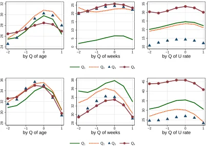
Education Misalignment. In figure 4 we report the results of the exercise for the misalignment
in education. In terms of age effects for the employed, the upper left panel (labeled by Q of age) show that applications occur more frequently for middle groups (Q2 and Q3) and the inverted U of the latter is much flatter for Q4, that is, the older employed seekers comply less to educational
requirements than younger groups. As for the unemployed, we observe in the lower-left panel that Q1 is different from the others: younger workers apply less to jobs for which they are overqualified
in terms of education. The peak of the Q1 group is slightly above zero, in contrast to the other groups which peak slightly below zero. Moreover, the application probability declines more sharply
for underqualified jobs (to the right of the peak). Except for the younger group, unemployed job seekers behave similarly regardless their age. The employed, in contrast, show higher intensity and less requirement compliance as they age.
In the upper center panel of figure 4, the application probability is substantially lower for Q1, the group with lowest tenure. The inverted U shapes peak in a positive misalignment level for Q1
and Q2, workers with tenure below the median, suggesting a job ladder motive of seekers applying for jobs for which they are underqualified in terms of education. For Q3 and Q4, the curve peaks roughly at zero, showing that employed workers seem less daring as they remain employed longer.
For the unemployed, the lower center panel of figure 4 portrays a downward displacement of the application probability curves as quartiles contain longer unemployment durations, especially when
workers are overqualified in terms of education. Curves Q2 and Q3 peak slightly to the left of zero, suggesting a conservative searching strategy that probably intends to secure a job.
The upper right panel depicts curves of the application probability of the employed as the unemployment rate increases (aggregate conditions worsen). The scale of the panel reveals that a higher unemployment rate affects application probabilities in a non-monotone way. Except for the
left part of Q4, all displacement seem mostly parallel, which suggests that business cycle conditions affect, on average, the intensive margin of search on the job. The right-lower panel depicts the
application probabilities for the unemployed. Employed and unemployed show a similar pattern as there is a non-monotone response to the cyclical conditions. Here, when unemployment is at its
highest (Q4), application probabilities increase as much as 20% with respect to Q3. However, the shapes of the curves for the unemployed show a slightly lower decline to the left of the peak of Q1. This is consistent with unemployed workers applying less to jobs for which they are overqualified
in terms of education.
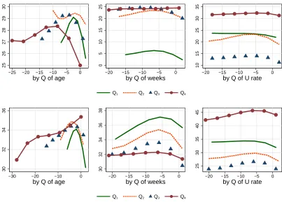
Experience Misalignment. The case of misalignment in experience is displayed in figure 5. In
the left two panels we observe that there are significant effects of age on how individuals align themselves with experience requirements: as we increase the age of workers, they have increasingly
25 26 27 28 29 30
−25 −20 −15 −10 −5 0
by Q of age
0 5 10 15 20 25
−20 −15 −10 −5 0
by Q of weeks
10 15 20 25 30 35
−20 −15 −10 −5 0
by Q of U rate
Q1 Q2 Q3 Q4
30
32
34
36
−30 −20 −10 0
by Q of age
30
32
34
36
38
−20 −15 −10 −5 0
by Q of weeks
25
30
35
40
45
−20 −15 −10 −5 0
by Q of U rate
[image:24.612.104.507.76.365.2]Q1 Q2 Q3 Q4
Figure 5: Predicted application probabilities for EMPLOYED (first row) and UNEMPLOYED (second row), given results from eq. (3) and different levels of misalignment in EXPERIENCE (see main text for details). The rest of regressors are at their sample means. The figure shows results when we split the sample in quartiles of age, weeks in the current labor force status and the national unemployment rate.
they are largely overqualified in term of experience.
In the two central panels, we depict the effect of experience misalignment by duration in em-ployment status.20
Employed workers who have recently started a job (Q1) apply substantially less
than the rest. Only those with tenure below the median (Q1 and Q2) seem somewhat sensitive to the experience requirement. The unemployed apply less and become less sensitive to requirements as their job search spells progress. We also observe that the maximum point in each curve shifts
to the left for longer spells, suggesting than the unemployed become increasingly overqualified in terms of experience as the elapsed job search increases.
Again, the right two panels of figure 5 display the effect of aggregate conditions. For the employed (top right panel), the average sensitivity to experience misalignment is quite low, as the
Q1 curve looks flat. For higher unemployment rates (Q2 and Q3) the inverted-U pattern become more apparent. However, when unemployment rate is high (Q4) the overall application probably increases despite the experience mismatch. For the unemployed, the effect is similar in the intensive
margin, but the curves show a greater sensitivity to experience misalignment compared to
on-the-20
job seekers.
15
20
25
30
35
−1.5 −1 −.5 0 .5 1
by Q of age
−10
0
10
20
30
−1.5 −1 −.5 0 .5 1
by Q of weeks
0
10
20
30
40
−1.5 −1 −.5 0 .5 1
by Q of U rate
Q1 Q2 Q3 Q4
25
30
35
40
−1 −.5 0 .5 1
by Q of age
25
30
35
40
−1 −.5 0 .5 1
by Q of weeks
20
30
40
50
−1 −.5 0 .5 1
by Q of U rate
[image:25.612.107.509.103.386.2]Q1 Q2 Q3 Q4
Figure 6: Predicted application probabilities for EMPLOYED (first row) and UNEMPLOYED (second row), given results from eq. (3) and different levels of misalignment in LOG-WAGES (see main text for details). The rest of regressors are at their sample means. The figure shows results when we split the sample in quartiles of age, weeks in the current labor force status, and the national unemployment rate.
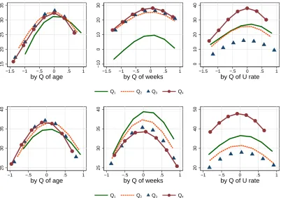
Wage Misalignment. Figure 6 shows results when we consider the (log) wage dimension. From
the results in the left panels, we observe that inverted U curves are similar for employed and
unemployed. The curve for the youngest employed group is slightly shifted to the right, suggesting a more daring behavior. For the unemployed, the youngest group also seems slightly less sensitive to log wage misalignment .
In terms of labor market state duration, we observe that the Q1 curve for the tenure of the employed is roughly a parallel downward displacement of the other curves in the graph. Hence, the
relative sensitivity to the gap of expected versus offered wage remains constant as tenure increases. The story is different for unemployed workers: they apply less as the job search duration increases
(shift down of the curves), and are increasingly more likely to apply to jobs offering wages lower than their expectations (less steep decline of probabilities for negative values of misalignment ). This behavior is consistent with a decrease in reservation wages, in line with findings in Krueger
Sensitivity to the offered-expected wage gap remarkably changes over the business cycle for
the employed. In a booming labor market, with low unemployment rate, probability curves are shifted to the right suggesting that employed workers follow more aggressive or daring plans (Q1 and Q2 in the upper-right panel). In a weaker market, the employed apply less and become
more conservative (Q3). However, in the weakest part of the cycle (Q4), the intensive margin increases a lot and the employed become somewhat more conservative as their curve peaks around
zero. Nevertheless, a large drop in the likelihood of applying suggests that on-the-job seekers have higher distaste for low-paying jobs when the unemployment rate is high. For the unemployed,
the story is similar, in the sense that wage misalignment curves slightly shift to the left as the unemployment rate increases. However, the relative distaste for low-paying jobs is slightly higher when the unemployment rate is low (Q1). These ideas are qualitatively consistent with theories
showing that labor market conditions affect wage formation. Unlike standard search and matching models, the wage adjustment seems to occur ex ante, as job seekers change their application behavior
targeting jobs paying less than they expect as labor market conditions worsen.
15
20
25
30
0 2 4 6 8
by Q of age
−10
0
10
20
30
0 2 4 6 8 10
by Q of weeks
0
10
20
30
40
0 2 4 6 8 10
by Q of U rate
Q1 Q2 Q3 Q4
20
25
30
35
0 2 4 6 8
by Q of age
20
25
30
35
40
0 2 4 6 8
by Q of weeks
10
20
30
40
50
0 2 4 6 8
by Q of U rate
[image:26.612.103.508.330.617.2]Q1 Q2 Q3 Q4
Location Misalignment. In figure7we present the results for distance misalignment , measured
in hundreds of kilometers in the horizontal axes. For employed workers, the oldest quartile (Q4) shows a remarkably larger likelihood to apply to jobs located far from their residence. The unem-ployed, on the other hand, show the same kind of distaste for distance of the job regardless of their
age. In all cases, greater distance can account for a large drop in the probability of application, as also shown in figure3.
When slicing the data by quartile of tenure, we observe that on-the-job seekers become increas-ingly insensitive to distance with longer tenures. It is notorious the large jump between Q1 and Q2.
For the unemployed, as the unemployment duration increases, we observe the opposite. The longer the unemployed search, the less likely they apply to more distant jobs. The decreasing distaste for distance is progressive, except for a mild reversion between Q3 and Q4.
Cyclical patterns affect the applicant sensitivity to distance as we show in the right panels of figure 7. Among the employed, the distaste for distance is larger when the unemployment rate
is low (Q1 and Q2). For the unemployed, the lower-right panel shows a steeper decrease when unemployment rate is high (Q3 and Q4).
−14
−12
−10
−8
1 2 3 4
quartile by Q of age
−13
−12
−11
−10
−9
−8
1 2 3 4
quartile by Q of weeks
−13
−12
−11
−10
−9
1 2 3 4
quartile by Q of U rate
[image:27.612.106.511.351.488.2]Employed Unemployed
Figure 8: Predicted effect of applying to an ad with occupation mismatch for EMPLOYED and UNEM-PLOYED given results from eq. (3). The other regressors are at their sample means. The figure shows results when we split the sample in quartiles of age, weeks in the current labor force status and national unemployment rate.
Occupation Misalignment. Figure8shows the point estimate of the misalignment coefficient on
required occupation being different from the individual’s occupation, by quartiles of time-domain
variables. The left panel first shows that occupational misalignment distaste is larger for the unemployed. As workers age, in both employment states the distaste decreases. This finding
shows that the unemployed are more tied to their occupations. Since workers without a specific occupation are classified in a “non declared” category, the estimated distaste may be partially
many occupations disappearing and others arising (Acemoglu and Autor,2011;Cort´es, Jaimovich,
and Siu,2017).
As tenure increases, the likelihood of applying to different occupations increases. The same occurs for the unemployed as their jobless spell increase, although for the long-term unemployed
(Q4) there is mild increase in occupational switch distaste.
Attempts at occupational mobility for the employed are higher for more neutral labor markets
(Q2 and Q3) than for strong or weak conditions (Q1 and Q4). This suggests that occupational reallocation is more difficult at the highest and lowest part of the business cycle. For the
unem-ployed, occupation mobility is accentuated (lower distaste) during weaker labor markets (Q3 and Q4). Therefore, occupational adjustments seem more likely in recessions as the unemployed apply more for jobs involving an occupational switch, and the employed apply less, making it easier for
the unemployed to find jobs. This finding is related to Carrillo-Tudela and Visschers (2014), who find that a significant share of unemployed in the PSID return to work in a different occupation
than the one they started unemployment.
Selective Margin and Gender.
As discussed above, females apply to more job positions in the website. However, when we control for observables, the gender margin reverses: other things equal, men apply more at the margin. In this section we seek to expand on this evidence and to show in which dimensions these gender
differences are more pronounced.
Figure 9 shows that for the employed, the male inverse-U curve is flatter suggesting a lower
sensitivity to the educational requirement, especially when overqualified (negative misalignment ). For the unemployed, we observe that the right part of the male curve decreases more markedly,
showing that male on-the-job seekers are much more reluctant to apply to jobs when they are underqualified in the education requirement. The evidence points at males having a wider search scope: they apply more than females to jobs below their educational level when employed, and to
jobs above when unemployed.
In the second row of figure 9, we observe gender differences the application probabilities as
a function of experience misalignment . The male inverse-U curves show a noticeable decrease when approaching zero, especially for the employed. Our interpretation is that males have a particular distaste for jobs for which they are not substantially more experienced than the posted
requirement. This feature is particularly strong for employed male job seekers. Since a higher experience requirement is often related to higher hierarchy or seniority, this hints at males searching
more than females for jobs that are higher in the job ladder.
In the third row of figure9we see little gender differences when applying for jobs offering wages