1973 Household Budget Survey: special features and results

1973 HOUSEHOLD BUDGET SURVEY SPECIAL FEATURES AND RESULTS

D. C. Murphy

(Read before the Society, May 20,1976)

INTRODUCTION

The first report on the large scale national Household Budget Survey (HBS) conducted by the Central Statistics Office (CSO) during 1973 was published earlier this month. It is, therefore, particularly opportune to have been invited by the Society to read a paper to-night on the HBS. At the outset I will briefly trace the historical development of these surveys and discuss some of the interesting methodological features of the 1973 national inquiry. After a brief look at the published results of the 1973 results I will examine the changes in Irish expenditure patterns over time and make comparisons with the results of a similar inquiry in the UK. I will then illustrate some important uses of the 1973 results by examining special categories of households (e.g., pensioner, family units), by consider-ing the updatconsider-ing of Consumer Price Index (CPI) weights and by providconsider-ing preliminary estimates of expenditure elasticities. I conclude by summarising the current position of the HBS and its future development.

PREVIOUS HOUSEHOLD BUDGET SURVEYS

1922 Survey

The 1922 survey is now only of historical and academic interest. Because of the disturbed state of the country and other reasons only 308 usable returns were collected. The results were used to weight the first index of consumer prices for this country . A further survey was planned for the end of the 1930s to update the index weights, but this had to be postponed because of the abnormal expenditure patterns during 1939-45 and subsequent years. By 1951 household consumption was considered to have stabilised into post-war patterns and a comprehensive HBS was initiated by the CSO in January, 1951 and con-tinued until September, 1952.

1951-52 Survey

The 1951-52 HBS was the first survey of household expenditure and income conducted in this country using modern sample survey techniques. Fieldwork was restricted to urban areas and was conducted by full-time and voluntary field personnel. The total number of household returns ultimately usecl was 12,300; these consisted mainly of sets of four returns made by a random sample of approximately 3,700 households covering a period of one week in four consecutive calendar quarters. The correlation resulting from the use of separate returns from the same household meant that the sampling errors of the derived estimates were higher than those which would have been obtained if 12,300 independent household returns had been used. This approach did simplify field work and ensured very high response in the second and subsequent quarterly fieldwork cycles. However, the most significant feature of the 1951-52 was that it pioneered the use in this country of questionnaires and expenditure diaries for data collection purposes. This interview/diary approach has been basically retained unchanged to-date.

1965-66 Survey

The 1965-66 HBS was again restricted to urban areas. Fieldwork extended from Sept-ember, 1965 to October, 1966 and was conducted by a team of full-time field personnel. A total of 4,759 household returns were realised; these consisted mainly of sets of two returns (including diary records for a period of fourteen consecutive days) completed by a sample of approximately 2,400 households at a six-month interval. The organisation of the survey into two separate six-month cycles again facilitated field work but, as in 1951-52, the sampling errors of the derived estimates were increased because of the correlation between the first and second cycle returns made by the same household.

1973 HOUSEHOLD BUDGET SURVEY

Principal Features

trad-itional combination of household questionnaires, personal questionnaires and personal expenditure diaries was used to collect the household expenditure and income data.

The most significant feature of the survey was the inclusion of rural as well as urban households for the first time in an Irish survey of this type. The 1973 results are, therefore, of particular interest because they give expenditure patterns for all households in the State and provide a basis for the first ever comparison of urban and rural standards of living. The extent of these differences can be examined in the first summary report on the 1973 survey published earlier this month. This initial report is summary only in the sense that household expenditure is summarised under 54 headings in most constitutent tables. The report is, in fact, comprehensive in scope since the results are classified in respect of all the most important household characteristics for the State (as a whole), urban areas, rural areas and rural farm households. One table was incorporated in the initial report summarising household expenditure patterns for these four classes of households under 341 individual expenditure headings. This represents the maximum expenditure detail coded in the 1973 HBS. Further reports on the 1973 survey are planned. These will relate to the State (as a whole), urban and rural areas, respectively, and will contain the detailed information on expenditure patterns together with estimates of average household income accruing from different sources.

Methodology

The methodology of the 1973 HBS was basically identical to that used in the 1965-66 urban survey; it is described in some detail in the initial report. However, I shall briefly discuss certain aspects of the rural coverage since it was undertaken for the first time in 1973 and presented serious methodological and practical problems particularly in respect of the estimation of farming income. The problems involved in extending the traditional urban coverage of earlier surveys to include rural areas had been the subject of research and investigation by Sheehy and O'Connor during 1970-71. The basic conclusion reached by Sheehy and O'Connor was that extension of the HBS to rural areas was feasible, but that farming income in the case of:

(a) small farms could be accurately estimated on the basis of data collected on a single visit;

(b) medium-to-large farms could only be accurately estimated using detailed farm accounts maintained by experienced Farm Surveyors for a full accounting year. This conclusion was accepted by the CSO and the 1973 HBS was designed accordingly. Analysis of farm activity levels and the available resources indicated that the delineation between small and medium-to-large for this purpose would have to be set at 30 acres. It was appreciated that the level of activity on some medium-to-large farms defined in this fashion would not be sufficient to justify the maintenance of detailed accounts; equally well it was realised that certain small farms would be so intensely worked that accurate estimates of their farming income would require detailed accounts. Subsequent events proved this point, but the number of latter cases encountered was not sufficient to significantly effect the estimation of average farm income.

most held agricultural degrees or diplomas. The Farm Accounts Books were designed along the lines of those used in the National Farm Survey conducted by the CSO during 1955-56, 1957-58.

The Farm Surveyors were appointed at an early stage so that they would initiate Farm Accounts on the specified quota of medium-to-large farms as early as possible. Individual Surveyors were intented to handle between 150 and 180 separate accounts, the number varied because allowance had to be made for differences in the geographic dispersal of individual assignments of survey areas. These areas were systematically surveyed during the successive cycles of farm accounts visits made to co-operating farms. Farm Surveyors visited each of these farms on at least four separate occasions during the twelve months accounting period.

The initial cycle of farm accounts visits lasted approximately five months since Farm Surveyors were not familiar with their areas, had to canvass the co-operation of the re-quired sub-quotas of medium-to-large farms for the survey as a whole (i.e., both the farm accounts and household budget phases), and had to complete the opening inventories of stocks, products, supplies, etc. in each co-operating case. Household Interviews subseq-uently called (one to twelve months later) on these medium-to-large farm households to complete the standard household budget part of the survey - i.e., collection of expenditure and non-farm income data. The second and third cycles of farm accounts visits took ap-proximately three and a half months to complete, these were concerned only with up-dating individual farm accounts. The closing inventory'visits were made twelve months after the initiation of accounts and took approximately four months to complete. Close liaison was maintained by the Household Interviewer and Farm Surveyor visiting the same household. The Surveyors secured the co-operation of these medium-to-large farm house-holds and were, therefore, able to identify their location for the Interviews and also advised them beforehand on the situation and problems which they would encounter.

The farm accounts phase of the 1973 HBS was quite successful. Some farmers dis-continued participating in the maintenance of accounts during the twelve months ac-counting period. In cases where the household phase of the survey had been completed the household was treated as co-operating and its farm income was estimated from the partial accounts. In cases where the Household Interviewer had not yet called the house-hold was eliminated. In neither case was it possible to introduce substitute medium-to-large farm households since there would not have been adequate time to maintain ac-counts for a full twelve month period. There were also instances where, although it was possible to have accounts completed, it was not possible to complete the household budget portion of the survey. In these instances the household was treated as a non-respondent for HBS, but the Farm Surveyor generally completed the farm accounts since these accounts are also being analysed separately for agricultural statistics purposes. In all, Farm Surveyors canvassed the co-operation of a random sample of 1,905 medium-to-large farms of which 1,146 (60 percent) agreed initially to participate in both the farm accounts and household budget phases of the HBS. A total of 927 (49 percent) satisfactorily com-pleted sets of household and farm accounts were ultimately realised for the HBS.

and farm accounts phases of the survey in rural areas at a minimum cost; it is described in detail in the published report. Farm Surveyors worked only in "country" survey areas which covered towns with less than 1,000 inhabitants and rural areas. Small farm house-holds in these areas were dealt with by the Household Interviewer, who obtained the required farm income details on a special interview questionnaire along with the household budget particulars she normally collected. Household Interviewers also handled all farm (small, medium or large) households in "urban" survey areas (i.e., located in towns with 1,000 inhabitants or more) in the same manner. A total of only 61 co-operating farm households were, however, surveyed in urban areas. Household Interviewers also had to ensure that the home consumption of farm or garden produce was accurately accounted for by the housewife and, although practical problems were encountered, this aspect of the survey did not present serious difficulties. Cost considerations present the major prob-lems in rural surveys of any type. In the 1973 HBS the relative urban and country survey area field costs per completed return from co-operating household were estimated to be of the following order:

Sample Divisions Relative Cost

per return (a) "Urban" survey

area:-Average household 1.0

(b) "Country" survey

area:-Household - no farm accounts 1.4 Household - with farm accounts 5.7 Average country household 2.5

These figures show that, given the extra travelling involved, the average field cost of sec-uring a completed return from co-operating households with no farm accounts in country survey areas was approximately 40 percent higher than the equivalent cost in urban areas. The maintenance of farm accounts was a very expensive operation and in such cases the average field costs per co-operating houshold were approximately six times the average urban cost. When the farm accounts field costs were averaged over all co-operating house-holds in country survey areas the average cost per return was still two and a half the aver-age cost per return in urban areas. To put these figures in true perspective it is estimated that the 1973 national sample could have been increased by 3,400 households for the cost of 927 completed farm accounts secured in the country survey areas.

Non-Response and Correction by Reweighting

far as possible for any over-or under-representation of particular types of households re-sulting from differential response rates (or possibly from the operation of the sampling plan).

Despite considerable publicity coupled with the payment of a gratuity of £1 to each person aged fifteen years and over and the use of full-time Interviewers the overall respon-se was 57 percent which was disappointing. Responrespon-se actually varied from 49 percent for the medium-to-large farms (who participated in both the household budget and farm accounts phases of the survey), 71 percent for other households in country survey areas; and 52 percent for urban areas. The urban response was substantially lower than the equivalent response rate of 66 percent achieved in the 1965-66 urban survey. This would indicate that there had been significant deterioration in the willingness of the public to participate in this type of comprehensive survey relating to personal matters. Reliable in-formation on differential response is very limited. The response rates quite clearly show the rural households were far more co-operative than their urban counterparts. The low response for the medium-to-large farm households is of course, explained by the fact that they were asked effectively to participate in two separate surveys (i.e., provision of house-hold and farm accounts data).

The reweighting process used to correct for differential response is described in detail in the published report. The household frequencies within detailed sub-classifications of the sample were effectively adjusted to conform with the corresponding 1971 Census distribution of households. The following characteristics were used to specify the detailed sub-classifications of households which were separately adjusted:

(a) Urban households - household size, town size and social group of head of household;

(b) Rural non-farm households - household size, provincial location and social group of head of household;

(c) Rural farm households -household size, provincial location and acreage farmed.

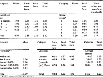
The proportional adjustments effected by the reweighting process within each of the sub-classifications distinguished in this fashion are specified in detail in the published report. However, they are conveniently summarised in Table 1 so that the basic underlying adjustments made are more readily distinguishable. The greatest increase in weighting was necessary in respect of rural farm households which were under-represented in all acreage classes. This was principally due to the fact that any medium-to-large farm which dropped-out of the maintenance of farm accounts could not be substituted for. The under-representation was not very pronounced for large households. Urban households consist-ing of a relatively small number of people, those in social groups* 1,2,6 and those locat-ed in the Dublin region and in the small towns under 1,500 inhabitants were also under-represented. On the other hand, without reweighting there would have been a serious over-representation of rural non-farm households. This over-representation was due to the fact that in instances where the co-operation of the specified sub-quota of medium-to-large farms had not been realised by the Farm Surveyor (due to refusals or drop-outs) the relevant Interviewer still tried to achieve the required overall area quota of 28 completed returns by securing the co-operation of other households.

Table 1: Proportional adjustments effected by weighting in 1973 HBS.

Category Urban Rural non-farm

Rural farm

Total State

Category Urban Rural non-farm

Total urban and

non-farm households Household

size 1-2 persons 3 4 . 5-6 .. 7+ ..

Total

Category

Town size**

Dublin and Dun Laoire

1.03 1.01 0.96 0.88

0.99

Towns 10,000+ Towns 1,500-5,000 Towns under

Total

1,500

0.91 0.93 0.83 0.77

0.88

Urban

1.06 0.86 0.89 1.14

0.99

1.36 1.06 1.20 1.03 1.09 0.96 1.13 0.90

1.22 1.00

Category

Location

Leinster Munster Connacht (pt.) Ulster

Total

Rural non-farm

0.85 0.89

0.90

0.88 Social group*

1 2 3 4 5 6

Rural farm

1.37 1.20

1.16

1.22

1.02 1.04 0.85 0.91 0.97 1.19

Total rural

0.99 1.03

1.04

1.02

1.06 0.86 0.64 0.80 0.73 1.06

Category

Acreage farmed

0-30 30-50 50-100 100+

Total 1.03 1.01 0.79 0.89 0.88 1.11

Rural farms

1.19 1.29 1.15 1.28

1.22 * Social groups defined in Table 4

** Including suburban areas as defined in 1971 Census of Population

The effect of the reweighting process on the sample frequencies is shown at the top of each table in the published report where both the actual and adjusted frequencies are provided. The overall effect of reweighting on the actual derivation of results is given in Table 2 which distinguishes weighted and unweighted figures for comparison purposes. As can be seen the disparities between the two sets of figures are not very substantial at these aggregate levels - for example, the average household expenditure for the State was reduced by only 2 percent as a result of the weighting process. However, an analysis along these lines extended to detailed sub-classifications could show much larger reductions or increases.

PUBLISHED 1973 HBS RESULTS

Principal Features

Table 2: Weighted and unweighted HBS results, 1973.

Item Description

Number of households in sample

Weighted No. 4,451 Urban areas Unweighted No. 4,451 Difference No. f

Weighted No. 3,297 Rural areas Unweighted No. 3,297 Difference No. Weighted No. 7,748 State Unweighted No. 7,748 Difference No.

Adjusted number of households in sample after reweighting

Household size

4,385 4,451 -66 3,363 3,297 +66 7,748 7,748

Males Females Total Household expenditure Food Alcoholic drink Tobacco

Clothing and footwear Fuel and light Housing

Household non-durables Household durables Miscellaneous goods Transport

Services and other expenses

Table 3: Summary of 1973 UBS results classified by urban/rural location.

Item Description Urban

areas No. 4,451 Rural areas Farm households No. 1,456 Other No. 1,841 All rural No. 3,297 State No. 7,748 Number of households in sample

Adjusted number of households in sample after re weigh ting

Household size Males Females Total 4,385 1.94 2.12 4.06 1,766 2.17 1.83 4.00 1,597 1.97 1.89 3.86 3,363 2.08 1.86 3.94 7,748 2.00 2.01 4.01

Weekly household expenditure Food

Alchohc drink Tobacco

Clothing and footwear Fuel and light Housing

Household non-durables Household durables Miscellaneous goods Transport

Services and other expenses

Total

Retail value of own

consumption (included above)

Table 4. Total average weekly household expenditure, 1973 classified by principal household characteristics*

Characteristics Urban

areas

Rural areas

State Characteristics Urban

areas Rural areas State All households Household size 1 person 2 persons 3 . 4 .. 5 .. 6 .. 7 .. 8 .. 9 .. 10+ ..

Gross weekly household income

Under £7

£ 7 and under £10 £10 .. £15 .. £20 .. £25 .. £30 .. £40 .. £50 .. £60 .. £70 .. £80 and over

£15 £20 £25 £30 £40 £50 £60 £70 £80 £ 45.04 £ 14.19 31.80 43.94 53.72 55.31 57.23 59.92 65.58 69.22 69.10 £ 9.28 14.12 18.29 22.85 29.54 32.58 40.60 50.82 57 38 64.56 72 15 88.80 £ 35.81 £ 10.75 22.76 33.60 41.27 45.88 49.52 57.64 64.37 60.02 65.90 £ 12.50 13.64 18.05 22.40 28.33 33.05 37.76 46.07 52.51 55.00 61.26 71.24 £ 41.03 £ 12.67 27.37 39.09 49.07 51.77 54.19 58.93 65.09 64.53 67.55 £ 11.00 13.84 18.16 22.59 28.92 32.80 39.53 49.23 ' 55.61 61.07 68.18 82.03 Planning region Eastern South Eastern South Western Mid-Western Western

Donegal & North Western

Midlands North Eastern Household tenure £ 48.77 38.64 42.21 41.27 40.07 39.00 36.79 47.85 £ £ 43.21 37.27 38.91 35.00 35.51 28.43 34.15 3151 £ £ 48.06 37.96 40.63 37.61 36.89 31.33 34.83 37 83 £ Owned outright Owned with mortgage Rented from Local Authority Rented other

Rent-free

Social group of head of household

1-professional, employer or manager

2-salaried employee and intermediate non-manual 3-other non-manual 4-skilled manual

5-semi and unskilled manual 6-farmers, agricultural workers

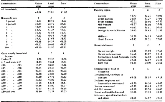
The expenditure patterns (summarised under 54 headings) for the State, urban areas, rural areas and rural farm households are classified by all important household character-istics. These are analysed in detail in the published report with particular attention given to the comparison of urban and rural patterns which have become available for the first time. Total average weekly expenditure for the principal sub-classifications of results given in the report are shown in Table 4 to demonstrate the underlying urban/rural diff-erences in the level of household expenditure. In interpreting expenditure totals and the breakdowns provided in the report due account should, of course, be taken of average household size with which the level of expenditure is directly related.

The distribution of households across the classifications in Table 3 and other classific-ations used in the survey is given by the adjusted number of households in sample after reweighting appearing at the top of each table. In some instances households were initially classified in greater detail than that published. For the convenience of users the percentage distributions of households in the State are given in Appendix 1 for the maximum detail sub-classifications of the following household characteristics*

Characteristics Detail distinguished on Appendix 1

(1) Household tenure 10 sub-classifications (2) Social group of head of household 12 ..

(3) Gross weekly household income 20 .. (4) Disposable weekly household income 20 .. (5) Gross weekly income of head of household 20 .. (6) Social welfare pensions As a % of gross 9 .. (7) Unemployment benefits weekly household 8 .. (8) Total state transfer payments income 10 ..

In the case of distributions involving households income it should be noted that income was understated to some degree in the survey. On average total recorded weekly household expenditure (£41.03) exceed the stated disposable weekly household income (£36.16) by some 13.5 percent. However, the bulk of this apparent deficit may be due more to the conceptual differences between the two figures and to the practical difficulties which some people (e.g., self-employed) had in quantifying their income, rather than due to the intentional understatement of income on a large scale. We can only surmise on this point as there is no way of determining the actual understatement or how its incidence varied with different types of households. No adjustments were made either to the stated or estimated incomes or to the ranges used for classification purposes. Consequently, it is possible that certain households have been assigned to slightly lower ranges than would have been appropriate if their true income was available. This would, of course, mainly effect households at the extremities of these ranges and, therefore, some tolerance must be attached to the specification of income ranges in the interpretation and use of the income distributions given in Appendix 1.

Total Expenditure of Private Households, 1973

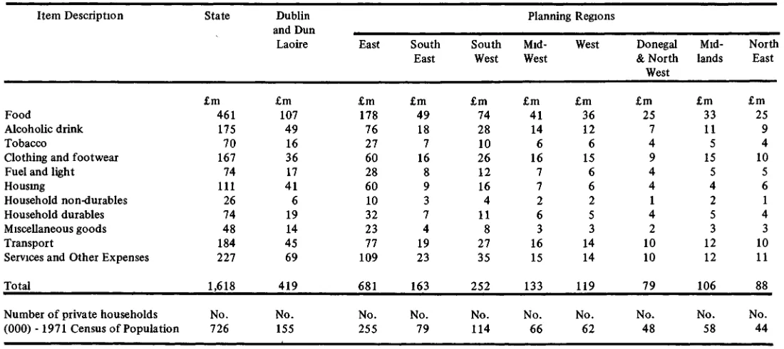
in 1973 by various household groupings. These estimated aggregates are given in Table 5 for the State as a whole, the Dublin metropolitan area and the Planning Regions. These estimates were compiled simply by grossing up the average weekly HBS expenditures for 1973 to an annual national basis using the total number of private households as given by the 1971 Census. To arrive at estimates of actual expenditure, the retail value of own farm/garden produce (i.e., non-cash consumption) was eliminated and the HBS figure for alcholic drink was adjusted to allow for the estimated 60 percent understatement of expenditure on the assumption that it was uniform in all sub-classifications.

The national aggregates tempts one to make a comparison with Personal Expenditure estimated annually by the CSO for the compilation of National Income and Expenditure Accounts. Even though such comparisons were made at item level within the CSO as part of process of validating the HBS results (this was how the 60 percent understatement of expenditure on alcholic drink was quantified) the State aggregates of household expen-diture given in Table 5 cannot be compared directly with the published 1973 Personal Expenditure figures because the two concepts differ radically in scope, coverage, concepts and nomenclature.

The scope of Personal Expenditure in the National Accounts covers the private con-sumption expenditure of all persons resident in "private" households and institutions (e.g., hotels, hostels, barracks, convents, etc.), together with the "collective" consumption (including wages/salaries paid to employees) of private non-profit institutions (e.g., schools, social clubs, private hospitals etc.). The coverage of Personal Expenditure in the National Accounts is restricted to consumption expenditure whereas household expenditure in the HBS includes some non-consumption items (i.e., in National Account parlance) such as mortgage repayments, insurance premiums, charitable and church donations, subscript-ions to clubs and societies, etc. There are conceptual differences as well - for example, the inclusion of the rental equivalent of owner occupied dwellings in National Accounts (actual housing expenses are covered in HBS) and the valuation of own consumption at producer prices (at retail prices in HBS). Differences in the classification of goods and services also exist at the moment. For example, the heading "food"- in Personal Expen-diture covers all food purchases including those by households in restuarants and hotels; the latter would be incorporated implicitly under the heading "hotel charges" in the HBS. These differences between HBS expenditure estimates and the Personal Expenditure figures compiled in the National Accounts have been considered at some length simply because they have not been highlighted previously in any published reports or com-mentaries.

Changes in Household Expenditure Patterns

Table 5: Aggregate Expenditure* (£ millions) of private households in 1973 classified by regional location (derived from 1973 HBS)m

Item Description

Food

Alcoholic drink Tobacco

Clothing and footwear Fuel and light Housing

Household non-durables Household durables Miscellaneous goods Transport

Services and Other Expenses

Total

Number of private households (000) -1971 Census of Population

State £m 461 175 70 167 74 111 26 74 48 184 227 1,618 No. 726 Dublin and Dun Laoire £m 107 49 16 36 17 41 6 19 14 45 69 419 No. 155 East £m 178 76 27 60 28 60 10 32 23 77 109 681 No. 255 South East £m 49 18 7 16 8 9 3 7 4 19 23 163 No. 79 South West £m 74 28 10 26 12 16 4 11 8 27 35 252 No. 114 Planning Mid-West £m 41 14 6 16 7 7 2 6 3 16 15 133 No. 66 Regions West £m 36 12 6 15 6 6 2 5 3 14 14 119 No. 62 Donegal & North West £m 25 7 4 9 4 4 1 4 2 10 10 79 No. 48 Mid-lands £m 33 11 5 15 5 4 2 5 3 12 12 106 No. 58 North East £m 25 9 4 10 5 6 1 4 3 10 11 88 No. 44

Table 6: Expenditure patterns of urban households in 1951-52,1965-66 and 1973.

Commodity group

Household size

Household expenditure Food

Alcoholic drink Tobacco

Clothing and footwear Fuel and light Housing

Household non-durables Household durables Miscellaneous goods Transport

Services and other expenses

Total

1951-52

4.15 persons

£

4.07 0.12 0.54 1.41 0.77 0.77 0.19 0.28 0.21 0.47 1.96x

10.79

%

37.7 1.1 5.0 13.0 7.1 7.1 1.7 2.6 1.9 4.4 18.1

100.0

1965-66

4.03 persons

£

6.70 0.79 1.31 1.93 1.12 1.72 0.35 0.87 0.59 2.04 3.82

21.22

%

31.6 3.7 6.2 9.1 5.3 8.1 1.6 4.1 2.8 9.6 17.9

100.0

1973

4.06 persons

£

13.15 2.18 1.93 4.27 2.18 4.15 0.77 2.16 1.56 5.17 7.54

45.04

%

29.2 4.8 4.3 9.5 4.8 9.2 1.7 4.8 3.5 11.4 16.7

100.0

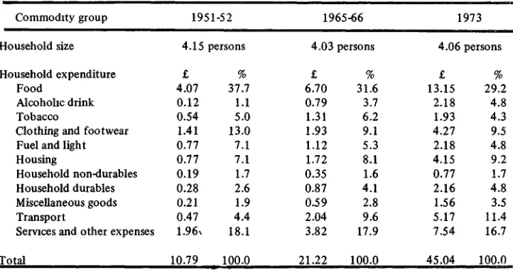
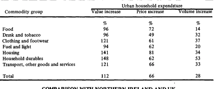
declined significantly; this was balanced by equally significant increases for housing, household durables, miscellaneous goods and transport. In making such comparisons al-lowance should, of course, be made for the effect on consumption patterns of the changes which occurred in the average size and composition of urban households over the period. Little significance can be attributed to the proportion of expenditure said to be spent on alcoholic drink because of possible variations in the degree of understatement. The most striking feature of Table 6 is, of course, the very substantial rise in the level of household expenditure since 1951-52. Much of this increase was due to corresponding increases in prices. Using the CPI to eliminate this price effect, the underlying volume in-creases in urban household expenditure are shown in Table 7. Using the commodity group indexes compiled in conjunction with the CPI it is also possible to examine the volume increases between 1965-66 and 1973 for particular commodity groupings. The CPI calculated to base mid-August, 1953 can only be used for this purpose. This does not allow the extension of the anlysis to the 1951-52 survey results and it also limits the com-modity break-down to the seven groups distinguished in that series. The results are given in Table 8 and show some interesting variations. Food consumption increased least of all in volume terms (only 14 percent); fuel and light also showed a relatively low increase in volume (20 percent). The large volume increase occurred in the case of household dur-ables (53 percent), whilst increases for other commodities ranged between 32 percent and 37 percent.

Table 7: Urban household expenditure volume changes between 1951-52 and 1973.

Periods

1951-52 to 1*965-66 1965-66 to 1973

1951-52 to 1973

Value increase

97

112

317

Urban household expenditure Price increase

64 66

170

Volume increase

20 28

Table 8: Urban household expenditure volume changes for commodity groups between 1965-66 and 1973.

Urban household expenditure Commodity group

Food

Drink and tobacco Clothing and footwear Fuel and light Housing

Household durables

Transport, other goods and services

Total

Value increase

% 96 96 121 94 141 148 121

112

Price increase

% 72 49 61 62 81 62 66

66

Volume increase

% 14 32 37 20 34 53 33

28

COMPARISON WITH NORTHERN IRELAND AND UK

Basis for Comparison

Surveys of household expenditure and income have been conducted on a continuing annual basis in the UK since 1957. The survey is titled the Family Expenditure Survey (FES) and the results have been used since 1962 to annually update the weighting basis of the UK Retail Price Index. The survey methodology is comparable to that used in the Irish HBS.

Between 1957 and 1967 only a small number of Northern Ireland households were in-cluded in the FES. However, since 1967 a separate inquiry has been conducted in the North based on an annual sample of approximately 900 households and separate results have been published. A random sub-sample of about 250 of these Northern Ireland house-holds is included in the overall sample of approximately 7,000 from which results are compiled in respect of the UK as a whole. Both the UK and Northern Ireland FES reports are available in respect of 1973° and this allows direct comparison with the 1973 HBS results.

Household Membership

In comparing the results of these Irish, Northern Ireland and UK surveys account must be taken of differences in household size and composition because of the close relationship which exists between these characteristics and the level and pattern of household expend-iture and income. The relevant particulars are given in Table 9 in respect of the households covered by each survey in 1973. Average household size in Ireland (4.009 persons) was significantly higher than that of Northern Ireland (3.320 persons) and of the UK as a whole (2.824 persons). Household composition was divided equally between males and females in all three regions. However, the average number of household members aged 65 years and over was 0.383 persons in this country; this was higher than the corresponding number in Northern Ireland (0.348 persons) and the UK (0.362 persons).

Expenditure Patterns

Table 9: Size and composition of the average household in Ireland, Northern Ireland and UK, 1973.

Average number of persons per household Persons Ireland Northern Ireland UK

No % No. % No. Sex

Male Female

Age

Over 65 years Under 65 years

Total persons " 4.009 100 0 3.320 100.0 2.824 100.0

Source HBS for Ireland, FES for UK

Table 10 Average weekly household expenditure in Ireland, Northern Ireland and UK, 1973. 2.002

2.006

0.383 3.626

49.9 50.1

9.6

90.4

1.607 1.713

0.348 2.972

48.4 51.6

10.5 89.5

1.379 1.445

0.362 2.462

48.8 51.2

12.8 87.2

Commodity group

Food

Alcoholic drink Tobacco

Clothing and footwear Fuel and light Housing

Household non-durables Household durables Miscellaneous goods Transport

Services and other expenses

Total

£

13.16 1.87 1.86 4.41 1.97 2.94 0.69 1.97 1.28 4.88 6.01

41.03

Average Ireland

%

32.1

4.6 4.5

10.9

4.8 7 2 1 7 4.8 3.1

11.9 14.6

100.0

weekly household expenditure Northern Ireland

£

10.26 1.44 1.68 4.10 2.49 3.22 0.69 2.52 1.05 6.08 4.81

38.34

%

26.8

3.8 4.4

10.7

6.5 8.4 1.8 6.6 2.7

15.9 12.5

100.0

£

9 63 1.85 1.47 3.48 2.17 6.51 0.70 3.09 1.52 5.37 7.07

42.86

UK

%

22.5 4.3 3.4 8.1

5.1

15.2 1.6 7.2 3.6 12.5 16.5

100.0

1973 in both absolute and percentage form for the ten commodity groups distinguished in the HBS. The classification of consumer goods and services in the FES differs some-what from that used in the HBS and the FES figures have been adjusted to ensure com-parability.

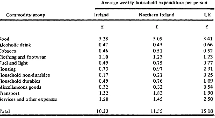
Table 11: Average weekly household expenditure per person in Ireland, Northern Ireland and UK, 19 73.

Average weekly household expenditure per person

Commodity group Ireland Northern Ireland UK

Food

Alcoholic drink Tobacco

Clothing and footwear Fuel and light Housing

Household non-durables Household durables Miscellaneous goods Transport

Services and other expenses

3.28 0.47 0.46 1.10 0.49 0.73 0.17 0.49 0.32 1.22 1.50

3.09 0.43 0.51 1.23 0.75 0.97 0.21 0.76 0.32 1.83 1.45

3.41 0.66 0.52 1.23 0.77 2.31 0.25 1.09 0.54 1.90 2.50

Total 10.23 11.55 15.18

Table 12: Percentage tenure distribution of private households in Ireland, Northern Ireland and UK, 1973.

Percentage distributions

Household tenure Ireland

Of

/o

47.7 23.4 16.0 10.8 2.1

Northern Ireland

Of 70

26.1 13.7 36.9 21.1 2.2

UK

Of /o

20.7 28.0 31.5 17.2 2.6 Owned outright

Owned with mortgage Rented - Local Authority Rented - private owner Rent free

Total 100.0 100.0 100.0

Other Features

The three 1973 surveys also permit the comparison of a number of other interesting feat-ures. For example, Table 13 shows the income distribution of private households in the three regions for the maximum detail common set of sub-classifications of Gross Weekly Household Income distinguished in each of the three reports. The comparison of these income distributions is, however, subject to a number of qualifications. In the first place, the definitions of Gross Weekly Household Income used in the HBS and FES are not id-entical; it is based on the concept of actual income on the occasion of the interview in the HBS and normal income in the FES. Furthermore, the distributions reflect the income of respondents which may have differed in the three surveys.

The incidence of certain household facilities and durable goods is also surveyed in these surveys. The relevant percentages for a common list of items are given in Table 14; Table 13: Estimated percentage income distributions of private households in Ireland, Northern Ireland

and U.K, 1973.

Gross weekly household income

Under £10 £10 and under £15 £15 .. .. £20 £20 .. .. £25 £25 .. .. £30 £30 .. .. £40 £40 .. .. £50 £50 .. .. £60 £60 .. .. £70 £70 .. .. £80 £80 and over

Total

Ireland

%

11.1 8.3 6.4 7.7 10.0 16.2 12.7 8.8 5.6 4.4 8.8

100.0

Percentage distributions of households

Northern Ireland

%

8.1 7.6 6.5 6.7 7.2 21.1 13.3 9.8 8.9 2.6 8.1

100.0

UK

%

4.2 8.7 6.5 5.3 5.5 13.1 14.4 13.2 9.4 6.7 13.0

100.0

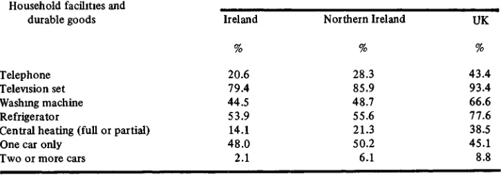
Table 14. Percentage incidence of certain facilities and durable goods in private households in Ireland, Northern Ireland and UK, 1973.

Household facilities and durable goods

Telephone Television set Washing machine Refrigerator

Central heating (full or partial) One car only

Two or more cars

Percentage incidence in private households

Ireland

%

20.6 79.4 44.5 53.9 14.1 48.0 2.1

Northern Ireland

%

28.3 85.9 48.7 55.6 21.3 50.2 6.1

UK

%

Table 15 • Percentage distribution of persons living alone in 1973 classified by age and sex.

Sex

Years of age Males Females Total % % %

Under 20 0.1 0.9 1.0 21 to 44 6.7 5.3 12.0 45 . . 6 4 18.4 20.3 38.7 65 and over 16.2 32.1 48.3

Total 41.4 58.6 100.0

Source 1973 HBS

they highlight some striking variations. With exception of cars, the percentage of house-holds with each of the items listed was substantially higher in the UK than in this country. Their incidence was also higher in Northern Ireland, but the differences were not as pro-nounced. The greatest Irish/UK disparities occurred in the case of telephones (20.6 perc-ent vis-a-vis 43 A percperc-ent) and cperc-entral heating (14.1 percperc-ent vis-a-vis 38.5 percperc-ent). The in-cidence of motor cars exhibited a different trend with 50.1 percent, 56.3 percent and 53.9 percent of the households in Ireland, Northern Ireland and UK, respectively, having one or more car. As would be expected, multi-car households were more plentiful in the UK and Northern Ireland than in this country.

1973 HBS RESULTS FOR SPECIAL TYPES OF HOUSEHOLDS

Households with Particular Compositions

The 1973 results were analysed by household size in the initial report, but households comprised of various combinations of adults and children* were not separately distin-guished. Household composition classifications are an important facet of the analysis of HBS results and they will be incorporated in subsequent detailed reports. To facilitate users in the meantime a summary State classification of the 1973 results by household composition is given in Table 16.

Variations in the absolute levels of total household expenditure can be seen to be directly related to household size and composition. However, the percentage expendit-ure distribution shows some interesting variations.

For example, in the case of two adult households there was a significant increase in the food percentage as the number of constituent children rose from 1 to 4+. The percentage expenditure on fuel and light and on housing was highest in single and two person house-holds. Perhaps the most intriguing feature of Table 16 is the almost consistent percentage, (i.e., 1.6 percent to 1.8 percent) of expenditure which households spent on non-durables within each composition category.

Table 16: Average household size and percentage household expenditure in the State, 1973 classified by household composition.

Item description

No of households in sample Adjusted number of house-holds in sample after reweighting

Average household size

Household expenditure Food

Alcoholic drink Tobacco

Clothing and footwear Fuel and light Housing

Household non-durables Household durables Miscellaneous goods Transport

Services and other expenses

Total

Total average weekly expenditure 1 adult No. 1,013 1,085 1.00 % 34.7 4.5 4.2 7.1 8.9 11.8 1.6 2.7 2.2 8.0 14.1 100.0 £ 12.67 2 adults No. 1,471 1,539 2.(JO % 32.3 5.4 5.1 8.7 6.2 7.7 1.6 3.7 2.9 11.5 15.0 100.0 £ 27.42 2 adults and 1 child 2

No. 378 375 3.00 % 27.3 4.3 3.7 8.8 4.7 9.2 1.7 6.7 2.7 16.2 14.7 100.0 £ 40.16 2 adults and children No. 513 511 4.00 % 27.6 3.9 3.1 9.4 4.7 11.1 1.6 6.3 3.3 12.3 16.6 100.0 £ 46.47 Household Composition 2 adults and 2 adults and 3 children 4+ children

tribution of persons living alone classified by both sex and age. As can be seen, over 48 percent of those living alone were aged 65 years and over, two-thirds of these were women. The expenditure patterns of men and women aged 65 years and over living alone are summarised in Appendix 2.

A selection of interesting household characteristics are analysed by household compos-ition in Table 17. The percentage household distribution is incorporated to show the relative importance of the different composition categories distinguished. The average age of the head of the household (HOH) is also shown and this can be taken as a rough indic-ation of the "maturity" of households. The incidence of washing machines, refrigerators, full central heating and cars showed similar trends, being high in households containing children and particularly low in single and two person households. The tenure distribution of households is also summarised for each composition category; this has a significant in-fluence on the level of housing costs. The single and two person households mainly lived either in owned-outright or rented accommodation, whilst the incidence of mortgaged and Local Authority rented dwellings was highest for households with children.

Typical Family Units

The expenditure patterns of households comprised of married couples with children are summarised in Table 18 for urban areas, lural areas and the State as a whole. Four types of family units are distinguished, namely,

(1) Married couple and one child; (2) .. .. .. two children; (3) .. .. .. three children; (4) .. .. .. four or more children;

The number of co-operating households in the original sample and the adjusted number after reweighting are shown for each of these four household categories in Table 18. The expenditure patterns of all households in the State is incorporated for comparison pur-poses.

The percentage expenditure spent on food was very low (i.e., 26 percent in urban and 28 percent in rural areas) for married couples with only one child, but it increased sub-stantially as the number of children in the family rose. However, for the other commodity groups the percentage expenditure spent by the four different types of families was sur-prisingly stable for the State as a whole. There were, of course, some significant differences between urban and rural areas, but these simply reflect the general disparities between urban and rural expenditure patterns revealed by the HBS. The significantly higher per-centage expenditure spent on food by rural families and the substantially lower perper-centage on housing are particularly noticeable. By comparison with urban households rural expen-diture figures for food include a relatively large proportion of home consumption of own farm or garden produce. The respective amounts are given in Table 18. The relatively low housing costs in rural areas are, of course, largely explained by the large proportion of families who owned their dwellings (see Table 19).

Table 17: Selected household characteristics, 1973 classified by household composition. as Household Composition 1 adult 2 adults

2 adults and 1 child 2 adults and 2 children 2 .. . . 3 .. 2 .. .. 4+ children

3 adults

3 .. with children

4 adults

4 .. with children

Other with children Other without children

State % Household distribution % 14.0 19.9 4.8 6.6 5.0 7.5 10.1 8.1 5.9 6.4 8.0 3.6 100.0 Washing machine % 8.0 22.9 45.5 63.3 78.0 79.9 32.4 62.8 48.4 65.2 65.6 51.4 44.5 Incidence Refrig-erator % 22.9 42.9 68.3 78.7 78.5 71.4 49.6 65.3 61.6 60.4 58.3 52.0 53.9 Full central heating % 2.5 7.1 21.5 27.9 29.1 20.8 5.7 13.3 5.0 10.4 8.5 4.1 11.1 Car(s) % 14.0 37.9 61.0 74.1 74.1 67.8 48.5 65.7 53.5 63.0 55.1 59.9 50.2 Owned outright % 55.2 57.8 34.3 26.3 26.6 31.1 59.5 46.6 54.4 45.0 43.0 56.6 47.7

% Tenure Distribution Owned with mortgage* % 9.0 16.2 28.3 42.3 44.0 31.6 18.8 28.6 21.5 26.5 26.1 24.9 23.4 Rented Rented other Local Authority % 12.8 10.5 11.2 15.4 20.0 29.0 10.6 20.3 13.5 21.5 25.8 11.7 16.0 % 17.8 13.5 23.4 14.2 7.6 7.0 9.4 3.2 9.3 5.1 4.3 6.7 10.8 Rent free % 5.1 1.9 2.8 1.8 1.8 1.3 1.6 1.3 1.3 1.9 0.8 2.1 Average age of HOH Years 61 - 60 38 36 37 3? 61 48 58 51 52 58 52

Table 18 :A verage household size and percentage household expenditure in urban/rural areas and State, 1973 classified by family type.

Item description

Number of households in sample Adjusted number of households in

sample after re weigh ting

Average age of HOH (years)

Household expenditure Food

Alcholic drink Tobacco

Clothing and footwear Fuel and light Housing

Household non-durables Household durables Miscellaneous goods Transport

Services and other expenses

Total

Total average weekly household expenditure*

*Includes consumption of own farm or garden produce

Couple and 1

Urban areas No. 249 247 36 % 26.2 4.8 3.6 7.8 4.6 11.5 1.8 6.2 2.8 15.3 15.4 100.0 £ 42.19 0.02 Rural areas No. I l l

109 40 % 28.3 3.4 3.9 11.2 4.7 4.0 1.6 8.4 2.3 19.1 13.1 100.6 £ 38.83 1.04 child State No. 360 356 37 % 26.8 4.4 3.7 8.8 4.7 9.3 1.7 6.8 2.7 16.4 14.7 100.0 £ 41.16 0.33

Couple and 2 children

Urban areas No. 371 369 35 % 25.8 4.1 3.0 9.1 4.6 12.9 1.6 5.9 3.1 12.1 18.0 100.0 £ 50.02 0.05 Rural areas No. 127 126 38 % 33.6 3.4 3.7 9.9 5.4 4.8 1.7 7.1 4.7 14.1 11.6 100.0 £ 37.32 1.60 State No. 498 494 36 % 27.4 4.0 3.1 9.3 4.8 11.2 1.6 6.1 3.4 12.5 16.7 100.0 £ 46.79 0.45 Couple Urban areas No. 288 282 36 % 28.6 4.1 3.4 7 6 5.0 11.4 1.7 6.4 3.5 11.9 16.4 100.0 £ 46.79 0.03

and 3 children

Rural areas No. 115 103 40 % 35.8 3.2 3.5 8.3 5.1 6.5 1.6 5.7 2.7 15.0 12.8 100.0 £ 41.12 1.84 State No. 403 385 37 % 30.3 3.8 3.4 7.8 5.0 10.2 1.7 6.3 3.3 12.7 15.5 100.0 £ 45.28 0.52 Couple Urban areas No. 409 384 37 % 32.1 3.5 3.6 7.9 5.2 9.6 1.6 5.5 3.2 12.2 15.6 100.0 £ 48.08 0.06

and 4+ children

Rural areas No. 208 190 41 % 38.1 3.0 3.4 10.3 4.7 6.3 1.6 5.3 2.2 13.1 12.1 100.0 £ 44.52 3.27 State No. 617 574 39 % 34.0 3.4 3.5 8.6 5.0 8.5 16 5.5 2.9 12.5 14.5 100.0 £ 46.90 1.13 All Households in State No. 7,748 7,748

• 5 2

Table 19: Selected household characteristics, 1973 classified by family type*

oo

Family Types

Couple and 1 child: Urban Aeas Rural .. State

Couple and 2 children* Urban areas Rural .. State

Couple and 3 children. Urban areas Rural .. State

Couple and 4+ children. Urban areas Rural State All households: Urban areas Rural .. State % Household distribution % 3.2 1.4 4.6 4.8 1.6 6.4 3.6 1.3 5.0 5.0 2.4 7.4 56.6 43.4 100.0 Washing machine % 49.0 42.2 46.9 66.3 57.0 63.9 79.9 74.4 78.4 84.8 71.4 80.4 51.7 35.1 44.5 % Incidence Refrig-erator % 70.9 67.1 69.7 83.1 69.1 79.6 83.5 67.6 79.2 75.3 63.8 71.5 64.1 40.6 53.9 Full central heating % 25.1 17.1 22.7 32.9 16.0 28.6 33.3 18.0 29.2 24.0 15.6 21.2 15.2 5.8 11.1 Car(s) % 57.6 75.9 63.2 72.2 83.1 75.0 71.3 84.2 74.8 66.8 72.6 68.8 48.2 52.7 50.2 Owned outright % 20.8 62.3 33.5 13.7 58.5 25.1 12.5 65.5 26.7 13.9 66.2 31.2 26.5 75.3 47.7

% Tenure Distnbution Owned with mortgage* % 34.2 16.0 28.6 51.2 20.5 43.4 53.4 19.2 44.2 40 0 14.5 31.6

3 1 7 12.7 23.4 Rented -Local Authority % 11.8 7.8 10.6 18.9 4.0 15.1 24.1 7.2 19.6 38.9 8.3 28.8 23.9 5.7 16.0 Rented other % 32.7 6.6 24.7 15.5 11.5 14.5 8.9 4.2 7.7 6.0 9.3 7.1 16.5 • 3.5 10.8 Rent free % 0.5 7.3 2.6 0.6 5.5 1.9 1.1 3 9 1.9 1 2 1.8 1.4 1 5 2.9 2.1

rural areas is also very noticeable when classified in this fashion by family type. The tenure breakdowns given in Table 19 show that the incidence of owner occupied ac-commodation for these four family units was below the national average in both urban and rural areas; this was balanced somewhat by a higher than average incidence of mort-gaged dwellings. The tenure pattern for rented accommodation is interesting. Privately rented dwellings predominated for families with one child, but the incidence of Local Authorities rented accomodation was substantially higher for the families with three or more children. Rural tenure patterns were, of course, dominated by the high incidence of owner occupied dwellings.

Households in Receipt of Social Welfare Payments

Being low income households the expenditure patterns of households in which income ac-crued mainly from social welfare payments would be expected to differ significantly from those of other households. To investigate this point two types of such households are dis-tinguished in Table 20, namely, those in which 75 percent and more of Gross Weekly Household Income was derived from:

(a) retirement, old age, widows and orphans social welfare pensions (these will be referred to as "pensioner" households';

(b) unemployment benefits and assistance, occupational injuries and disability bene-fits and redundancy payments (these will be referred to as "state assisted" house-holds).

It was considered that a cut-off point of 75 percent would be high enough to distinguish two relatively homogenous groupings of households, and sufficiently low to ensure that the corresponding sub-sample sizes would be adequate for estimation purposes.

Urban and rural households are separately distinguished for comparison purposes. The number of co-operating households in the original sample and the adjusted number after re weighting are also shown; these indicate the relative importance of the different cate-gories of households distinguished.

As expected the absolute level of total household expenditure was very low in "pensioner" households; this was due not only to their low income but also to their small size (1.52 persons on average). The total expenditure of "state assisted" households, al-though almost double that of "pensioner" households, was still substantially less than that of other households. The expenditure patterns of both "pensioner" and "state assisted" households were mainly characterised by high percentage expenditures on food, fuel and light; and by lower than average percentage outlay on household durables, miscellaneous goods and transport. The high proportion of expenditure spent on tobacco by "state ass-isted" households is particularly noticeable. The urban/rural breakdown reveals little of interest except the normal differences.

Table 20. Average household size and expenditure patterns of households in urban areas, rural areas and State, 1973 where 75% of gross household in-come was comprised of social welfare pensions and of State unemployment payments.

15% of gross hid income from social welfare pensions

75% of gross hid income from state unemployment payments

Other households All households

Item Description Urban areas Rural areas State Urban areas Rural areas

State Urban Rural State Urban Rural State areas areas areas areas

o

Number of households in sample Adjusted number of households in

sample after reweightmg

Household size Males Females Total

Average age of head of household (years)

Household expenditure Food

Alchohc drink Tobacco

Clothing and footwear Fuel and light Housing

Household non-durables Household durables Miscellaneous goods Transport

Services and other expenses

No. No. No. No. No. No. No No No. No. No. No 273 250 523 104 85 189 4,074 2,962 7,036 4,451 3,297 7,748

303 235 538 100 76 176 3,982 3,052 7,034 4,385 3,363 7,748

0.40 1.04 1.44 0.70 0.92 1.62 0.53 0 99 1.52 2 48 2 38 4 87 2 10 147 3.57 2.32 1.99 4.30 2.05 2.20 4 24 2.18 194 4 12 2 11 2 08 4.19 1.94 2.12 4 06 2 08 186 3.94 2.00 2 01 4 01

71.3 72.3 71.7 43.4 50.2 46.4 48 1 54 I 51.0 49 6 55.9 52.3

44.5 3.0 5.0 5.7 10.9 12.3 2.0 2.6 2.1 1.2 10.7 45.3 3.6 6.3 10 8 11.7 3.4 2.0 2.6 2 0 3.1 9.3 44.9 3.2 5.6 8.0 11 2 8.2 2 0 2 6 2.1 2 1 10 1 40 0 39 8 3 9.2 8 4 7 2 21 39 3.6 5 0 8.3 44 1 5.3 8 4 9 1 6 9 5.0 2 6 3.8 2 3 7.4 5.2

4 1 5 4.4 8.4 9.1 7.8 6 4 2.3 3.9 3.1 5.9 7 2 28 8 4 9 4.2 9.5 4.7 9.2 17 4.8 35 117 16 9 36 5 4 1 4 8 12 9 4.5 3 8 17 4 9 2 6 12 8 11.3 31.7 4.6 4.5 10 8 4 6 7.2 1.7 4.8 3.1 12.2 , 14 8 29.2 4 8 4.3 9 5 4.8 9 2 17 4 8 3.5 115 16 7 36.8 4 1 4 9 12.9 4.7 3 8 17 4 8 2.5 12 6 11.2 32.1 4 6 4 5 10.7 4.8 7 2 1.7 4.8 3.1 11.9 14.6 Total

Average weekly household

Table 21: Selected characteristics of households in urban areas, rural areas and State 1973 where 75% of gross weekly household income was comprised of social welfare pensions and of state unemployment payments.

Income composition

75% of gross household income from social welfare pensions

Urban areas Rural areas State

75% of gross household income from State unemployment payments

Urban areas Rural areas State Other households Urban areas Rural areas State All households Urban areas Rural areas State % Household distribution % 3.9 3.0 6.9 1.3 1.0 2.3 51.4 39.4 90.8 56.6 43.4 100.0 Washing machine % 12.8 4.9 9.4 33.5 12.4 24.4 55.1 38.0 47.7 51.7 35.1 44.5 % Incidence Refrig-erator % 28.3 15.5 22.7 30.1 17.8 24.7 67.7 43.1 57.0 64.1 40.6 53.9 Full central heating % 0.7 0.6 0.7 7.5 2.9 5.5 16.5 6.3 12.1 15.2 5.8 11.1 Car(s) % 1.6 5.4 3.3 13.4 28.6 20.0 52.6 56.9 54.5 48.2 52.7 50.2 Owned outright % 33.6 55.6 43.2 11.0 46.4 26.4 26.3 77.5 48.5 26.5 75.3 47.7

% Tenure distribution

Owned with* mortgage % 11.6 17.6 14.2 13.0 27.9 19.5 33.6 11.9 24.2 31.7 12.7 23.4 Rented-Local Authority % 31.4 12.3 23.1 61.2 15.5 41.4 22.4 4.9 14.8 23.9 5.7 16.0 Rented - other % 18.8 6.3 13.4 12.7 6.8 10.1 16.4 3.2 10.7 16.5 3.5 10.8 Rent free % 4.6 8.3 6.2 2.1 3.5. 2.7 1.2 2.4 1.8 1.5 2.9 2.1

owning their dwellings under mortgage were, in fact, participants in tenant purchases sch-emes operated by Local Authorities. The expenditure patterns of single persons and mar-ried couples living alone in receipt of social welfare retirement and old age pensions are summarised in Appendix 2 for those who may be interested in these particular types of households.

USE OF HBS RESULTS FOR CPI WEIGHTING PURPOSES

General Points

The most important use of the HBS results is to provide a basis for updating the weights used in the compilation of the CPI. New weights were introduced in calculating the index for mid-February, 1976 (to base mid-November, 1975 as 100). For this purpose the HBS expenditure pattern for all households combined was adjusted by:

(a) allowing for price changes between 1973 and 1975;

(b) incorporating a correction for the understatement of drink in the HBS;

(c) excluding the retail value of own farm and garden produce consumed in the home (since the CPI is based on the concept of current money expenditure of private households)*;

(d) excluding the capital repayment element of house purchase mortgage payments*; (e) excluding such items as church/charity contributions, personal cash allowances

and lottery/betting payments which either have no"price" or cannot be priced*.

The updated weighting basis relates to rural as well as urban households and includes mortgage interest payments for the first time.

Comparison of "Old" and "New" CPI Weights

It is of interest to compare the expenditure weights used in the compilation of the former CPI (base mid-November, 1968 as 100) with those of the updated series now being piled to base mid-November, 1975 as 100. The percentage urban weights used in the com-pilation of the former series are directly compared with the national (i.e., urban and rural) weights used in the present series in Table 22.

The CPI is compiled on the principle of pricing a "market basket" of fixed quantities of a representative selection of goods and services in successive quarters. In practice the index is calculated by updating on a quarterly basis the cost (i.e., expenditure weight) in the base quarter of each item in the "basket" by applying the percentage changes in prices between successive quarters. Thus the percentage distribution of these expenditure weights can alter over time directly as a result of prices changing at different rates. For this reason, the percentage expenditure weights of the former series are shown for both mid-November, 1968 (base quarter) and mid-November, 1975 (final quarter) in the first two columns of Table 22. The weights in the second column are those which would have been applied to price changes between November, 1975 and February, 1976 to calculate the quarterly percentage change in the CPI if no new HBS results had been available for *Those exclusions account for approximately 9 percent of the total stated average weekly household