Environmentally Aware Households

Munich Personal RePEc Archive

Environmentally Aware Households

Delis, Manthos and Iosifidi, Maria

Montpellier Business School, Montpellier Business School

12 February 2019

Online at

https://mpra.ub.uni-muenchen.de/92138/

Environmentally Aware Households

Manthos D. Delis

Montpellier Business School

Maria Iosifidi

Montpellier Business School

Environmentally Aware Households

Abstract

The rising environmental awareness induces a changing landscape for policymakers and real economic prospects. We examine the properties of a general equilibrium model with endogenous household preferences (for labor, consumption, and environ-mental quality) and a negative environenviron-mental externality. The endogeneity of labor creates an additional channel of substitution between environmental quality and labor, besides the channel of substitution between environmental quality and con-sumption. We show that a key requirement for improved output following a positive shock in the weight of environmental quality (household environmental awareness) is that environmental awareness trades off the weight on labor and not the weight on consumption. An interesting feature of the model is that the existence of the environmental externality gives a non-zero capital tax in the long run.

Keywords: Environmental awareness; Environmental quality; Labor; Consumption; Real

1. Introduction

What is the role of household environmental awareness on their consumption and

labor decisions? What are the implications of these decisions for the real economy? The

answer to these questions are important in light of increased pressure for environmental

quality and environmental awareness. For example, 94% of European citizens say, as of

2017, that protecting the environment is important to them, 81% suggest agree that that

environmental issues have a direct effect on their daily life and their health, and 87%

suggest that they have a personal role to play (Special Eurobarometer, 2017). Similar

results emerge from relevant questions in the six waves of the World Values Surveys.

From a more practical viewpoint, the Fukushima nuclear disaster in 2011 strengthened

considerably the share of people opposing the use of nuclear power (BBC, 2011). The

German government decided to shut down all nuclear plants by 2022, despite the obvious

impact of this decision on output and employment, especially given the surging economic

turmoil in the European Union during the same period. Such decisions place inevitably

the role of environmental awareness in a central position within the economic decisions

of households, the related fiscal decisions of governments, and the end results for real

economic outcomes.

We focus on the the weight economic agents place on environmental quality (henceforth

environmental awareness) vis-a-vis the respective weights on labor and consumption. Our

setup augments the Ramsey-type frameworks of Chamley (1986) and Judd (1985),

hence-forth Chamley-Judd, by adding an environmental externality to an economy in which

labor, consumption, and environmental quality are determined endogenously.

The representative economy consists of a large number of identical infinitely-lived

households, whose utility depends on private consumption, labor, and the stock of

envi-ronmental quality. The households consume, save, and produce a single good. Output

produced yields environmental pollution and this worsens environmental quality, which

is assumed to be a public good. In other words, private agents do not internalize the

and policy intervention is justified. A Ramsey-type planner (government) intervenes and

chooses the best competitive equilibrium for this problem.

The main novelty of our model is that both the labor-leisure decision of households and

their consumption are included in the consumer preferences. Indeed, to the best of our

knowledge, there is no other study that examines the interplay between an environmental

externality and labor-leisure decisions in a model similar to that of Chamley-Judd. Our

novelty is important for two main reasons.

First, our analysis allows examining the response of labor supply to changes in the

beliefs and attitudes of households with respect to environmental awareness. This is quite

important in light of the developments in many countries against production activities that

are particularly harmful for the environment. The response of many European countries

to the Fukushima disaster and the response of multiple labor unions even from the 1960s

further motivate our theoretical model, as they are suggestive of a reduced labor supply

to environmentally harmful jobs. This is a key finding of the recent empirical literature

(Iosifidi, 2016).

Second, the relation between labor supply and environmental awareness is possibly

related to the employees’ social status, i.e. the nature of the job is placing the employee

in a particular cast. This idea is central in theories of social stratification and class at

least since the times of Marx and Weber. In other words, as environmental awareness

increases, the labor supply linked to environmentally harmful activities is lower because

of the lower social status given to such production activities.

The Chamley-Judd result, which is particularly relevant for our analysis, states that

in a steady state there should be no wedge between the intertemporal rate of substitution

and the marginal rate of transformation, i.e. the optimal tax on capital is zero. In

our framework, individuals face two types of trade-offs, one between consumption and

environmental quality and another between labor-leisure and environmental quality. This

is mostly observed in the real business cycle (RBC) literature, where labor is endogenous,

and creates an additional choice for intratemporal substitution (see e.g., Kydland and

Our economy yields a unique steady state, which we shock to obtain the paths of

our endogenous variables. We are mainly interested in the parameters characterizing

the effect of household environmental awareness on environmental quality, as well as the

overall effect on output and welfare. We find that an increase in environmental awareness

always leads to higher environmental quality, irrespective of whether higher environmental

awareness comes at the expense of less weight on consumption or labor. For the effect

on output, the results are quite intriguing. We find that output (and consumption and

labor) decreases when the increases in environmental awareness comes at the expense of

the wight on consumption. In contrast, when environmental awareness increases at the

expense of the weight on labor, output increases.

We also show that the capital tax is determined in equilibrium, among others, by

the environmental parameter of our model related to pollution. More specifically, in

the case where the pollution externality is zero, the capital tax is also zero and our

result is identical to the Chamley-Judd result. In contrast, in the presence of a negative

environmental externality, the tax on capital is positive and the Chamley-Judd result does

not hold. We could say that in our model with an environmental externality, we obtain a

second-order Chamley-Judd result, where the capital tax is always positive. This result is

evident only in the literature imposing constraints on the government to impose taxes. In

our model, the mere existence of an environmental externality where labor, consumption,

and environmental quality are endogenous yields this result. The empirical implication

of this result is that a positive

The rest of the paper is organized as follows. In the next section we provide the

background literature implications on which we build our model. describe our model. In

Section 3 we describe the economy. In Section 4 we solve for the decentralized competitive

equilibrium, check for its stability, and compare our model with the equivalent model with

endogenous labor using impulse responses and stylized facts. In Section 5 we solve for the

planner’s problem and check for its stability. Moreover, we compare our result with the

Chamley-Judd result, offer some numerical examples, and illustrate the dynamic responses

2. Background

Our work is related to a flourishing literature on growth and environmental quality. In

this section, we aim to place our work within the most relevant macro literature. In a

sem-inal contribution, Bovenberg and Smulders (1995) were among the first to explore the link

between environmental quality and economic growth in an endogenous growth model that

incorporates pollution-augmenting technological change. Their model includes

environ-ment as a renewable resource. In particular, they model how technological improveenviron-ments

enable production to occur with lower levels of pollution and with more effective use of

renewable resources. They show that environmental quality and cleaner technology

repre-sent good reasons for policy intervention, as both have a public good character. Further,

the revenues from pollution taxes (or pollution permits) exceed public expenditures on the

development of pollution-enhancing technology and the optimal size of the government

budget tends to increase when environmental awareness increases.

Several other papers consider general equilibrium frameworks with pollution taxation.

Angelopoulos, Economides, and Philippopoulos (2013) rank different environmental policy

instruments under uncertainty. Xepapadeas (2005) proposes relevant models to study the

effects of environmental concerns on economic growth. The important assumptions in

these models relate to the choice of emissions in an optimal way and to the devotion

of resources to pollution abatement. Dioikitopoulos, Kalyvitis, and Vella (2015) study

the allocation of tax revenues between infrastructure and environmental investment in a

general-equilibrium growth model with endogenous subjective discounting. An interesting

finding of this paper is that, when environmental awareness increases, it is optimal for

governments to perform green spending reforms.

A common characteristic of these papers is that the utility function is independent from

the labor/leisure decision of households. This is quite important in our view, given the

movement over at least the last fifty years of households to demand higher environmental

quality and relevant jobs (Special Eurobarometer, 2017; previous versions). This implies

decision of households, in addition to the consumption decisions that are studied in the

literature. In fact, in the only empirical study on this issue, Iosifidi (2016) shows that the

link between environmentally-aware households and their labor supply is tighter compared

to the link between environmental awareness and consumption.

In the endogenous-growth literature with fiscal policy (but without environmental

quality) many studies indeed treat labor supply as inelastic. This treatment limits certain

aspects of fiscal policy (Turnovsky, 2000). More precisely, De Hek (2006) studies an

endogenous growth model with physical capital and suggests that the flexibility of the

labor supply induces agents to spend more or less time on leisure activities, depending on

the relative sizes of the substitution and income effects. Flores and Graves (2008) argue

that exogeneity of labor generally results in undervaluation of utility due to increases in

the provision of a public good. Phrased differently, if the labor supply is exogenously

fixed, the Le Chatelier-Samuelson principle holds. Intuitively, this follows from the fact

that an increase in the cost of the public good will result in a higher marginal valuation

of ordinary private goods, as their quantities are reduced to pay for the public good, and

this in turn will result in a higher marginal cost of leisure.

Our model is also related to the literature predicting the existence of a zero capital

tax rate in the long run. The seminal contributions in this literature are the studies by

Chamley (1986) and Judd (1985). In similar Ramsey-type settings, these studies show

that if an equilibrium has an asymptotic steady state, then the optimal policy is to set

the capital tax rate equal to zero. In other words, any positive capital income tax does

not help in any efficiency or redistributive goals in the steady state.

However, a more recent literature shows that the optimal factor taxation may involve

positive tax rates on both capital and labor incomes (e.g., Correia, 1996; Stiglitz, 1987;

Jones, Manuelli, and Rossi, 1997; Acemoglu, Golosov, and Tsyvinski, 2011). Debortoli

and Gomes (2012), examine the case where the choice between capital vs. labor income

taxation can be intrinsically related to the allocation of expenditure across different

pub-lic goods. In their model, taxing profits constitutes a way to extract the private rents

as opposed to the optimality of zero capital taxation in Judd (1985) and Chamley (1986).

Evidently, in all of these papers, a non-zero capital tax arises due to constraints on the

government to impose taxes. In our model these constraints are not needed; the mere

existence of an environmental externality where labor, consumption, and environmental

quality are endogenous yields this result.

3. Description of the economy

We describe our basic framework, placing particular emphasis on the fact that,

be-sides environmental quality, both labor and consumption decisions are endogenous in the

individual’s preferences and their weight in the utility function is proportional to the

weight placed on environmental quality. Subsequently, we describe the decisions of firms,

the laws of motion of natural resources, the resources constraint, and we close the model

with the government budget constraint. We model a Ramsey-type economy, assuming

in-tertemporal utility-maximizing households, and perfectly-competitive profit-maximizing

firms (Beltratti, 1996; Xepapadeas, 2005).1

3.1. Households

We assume that the population size is constant and equal to one. The representative

infinitely-lived household maximizes the intertemporal utility

∞

X

t=0

βt_U(c

t, lt, Qt), (1)

where cis the private consumption, l is leisure, Q is the stock of environmental quality,

1

and β ∈(0,1) is the time discount factor. The utility function has the form2_:

U(ct, lt, Qt) =

[(ct)µ1(lt)µ2(Qt)1−µ1−µ2]1−σ

1−σ , (2)

where µ1, µ2, µ3 = 1−µ1 −µ2 ∈ (0,1) are preference parameters that assign weights to

consumption, leisure, and environmental quality, respectively, and σ≥0 is the intertem-poral elasticity of substitution. We define the weight onQas “environmental awareness.” The household is endowed with one unit of time that can be used for leisure lt or labor

nt, thus nt+lt = 1. Each household can save in the form of capital kt, receiving a rate

of return rt. Also, households supply labor services and receive labor income wtnt.

Fur-ther, they receive dividends πt. Each household has to pay a portion of its income to the

government in the form of linear taxes. τk

t is the tax on capital income and τtl is the tax

on labor income. The flow budget constraint of the household is

kt+1−(1−δk)kt+ct=yt= (1−τtl)wtnt+ (1−τtk)rtkt+πt, (3)

where kt+1 is the end-of-period capital stock, kt is the beginning-of-period capital stock,

and δk _{∈[0,1] is the rate of capital depreciation.}

It follows that the household’s problem is to

max

{ct,lt,kt+1}∞_t=0

∞

X

t=0

βt[(ct)µ1(1−nt)µ2(Qt)1−µ1−µ2]1−σ

1−σ ,

s.t.kt+1−(1−δk)kt+ct= (1−τtl)wtnt+ (1−τtk)rtkt+πt,

taking wt, rt, Qt, and the policy as given. The problem expressed in a Langrangian form 2

is given by:

L=

∞

X

t=0

βt_{[(ct)µ1(1−nt)µ2(Qt)1−µ1−µ2]1−σ

1−σ

+λt[(1−τtl)wtnt+ (1−τtk)rtkt+ (1−δk)kt+πt−ct−kt+1]}.

The FOCs for this problem with respect to ct, nt, and kt+1 respectively are

Uct =λt, (4)

ct

1−nt

= µ1

µ2

(1−τl

t)wt, (5)

Uct =βUct+1[(1−τ

k

t+1)rt+1+ 1−δk]. (6)

The first equation gives the marginal utility of consumption and the second equation is

the FOC with respect to labor. The last equation is the Euler equation for capital. It tells

us that along an optimal path, the marginal utility from consumption at any point in time

is equal to the opportunity cost of consumption. More specifically, the Euler equation

says that, on the one hand, the household must be indifferent between consuming one

more unit today and, on the other, saving that unit and consuming in the future. If the

household consumes today, it gets the marginal utility of consumption today, i.e. the

left-hand side of the equation, Uct. If, in contrast, the household saves that unit, it gets

to consume [(1−τk

t+1)rt+1+ 1−δk] units in the future, each giving him Uct+1 extra units

of utility. Because this utility comes in the future, it must be discounted by the weight

β. That’s the right side of the Euler equation. The fact that these two sides must be equal is what guarantees that the household is indifferent to consuming today versus in

the future.

3.2. Firms

constant returns to scale of the form

yt=Akatn

1−a

t =f(kt, nt), (7)

where a∈(0,1) is the output elasticity of private capital and 1−a ∈(0,1) is the private elasticity of labor.3_{A is total factor productivity or the index of production technology,}

which is assumed to be constant. In each period, the representative firm takes wt and rt

as given4_{and uses capital and labor services from households. The objective of the firm}

is to

max

{lt,kt+1}∞_t=0

πt=yt−wtnt−rtkt. (8)

The FOCs for this problem are

rt=a

yt

kt

, (9)

wt = (1−a)

yt

nt

, (10)

so that π= 0.

3.3. Laws of motion of natural resources

The evolution of the stock of environmental quality is given by

Qt+1 = (1−δq) ¯Q+δqQt−pt+νg, (11)

where ¯Q ≥ 0 is the environmental quality without pollution, pt is the current pollution

flow, andδq _{∈[0,1] is the degree of environmental persistence. Moreover,gis the exogenous}

public spending that includes spending on abatement activities and ν ≥ 0 shows how

3

In our model, pollution does not enter the production function. There is a large literature that introduces pollution in the production function by assuming that pollution or environmental quality affects amenities and productivity (Brock, 1973; Xepapadeas, 2005; Aznar and Ruiz-Tamarit, 2005).

4

public abatement spending is transformed into units of renewable resources. The flow of

pollution is caused by the production of output and is given by

pt =φAktan

1−a

t , (12)

where φ is an index of pollution technology and reflects the emissions per unit of out-put.5_{Note that we assume a linear relation among economic activity, pollution, cleanup}

policy, and the change in natural resources (e.g., John and Pecchenino, 1994; Jouvet,

Michel, and Rotillon, 2005).

3.4. Government budget constraint

The government collects revenues from the taxes on labor and capital.6 _{On the}

ex-penditure side, it finances an exogenous stream of government purchases, {gt}∞t=0, that

include spending on abatement policy. Assuming a balanced budget, we have

gt=Akatn1t−a[aτtk+ (1−a)τtl]. (13)

3.5. Resource constraint (technology)

Output can be consumed by households, used to increase the capital stock, and/or

used by the government. Therefore, the resource constraint is

ct+gt+kt+1 =yt+ (1−δk)kt. (14) 5

We assume that the index of pollution technology is a parameter. Instead, we can assume that it depends on private or public investment in greener technology, or to follow a stochastic process. Our inferences do not change and we aim for the simplest approach.

6

4. Decentralized competitive equilibrium (DCE)

We solve the problem described in Section 3 for a Decentralized Competitive

Equilib-rium (DCE) in which (i) households maximize welfare, (ii) firms maximize profits, (iii)

all constraints are satisfied and, (iv) all markets clear. The DCE of the above economy is

given by the following equations:

ct

1−nt

= µ1

µ2

(1−τl

t)wt, (15)

Uct =βUct+1[(1−τ

k

t+1)rt+1+ 1−δk], (16)

Qt+1 = (1−δq) ¯Q+δqQt−φAktan

1−a

t +νgt, (17)

gt=Akatn1− a t [aτ

k

t + (1−a)τ l

t], (18)

ct+kt+1 =Aktan

1−a

t −gt+ (1−δk)kt. (19)

This is a four-equation system in {ct, nt, Qt+1, kt+1}∞t=0. The DCE holds for given

initial conditions for the stock variables k0 and Q0, the FOCs of the representative firm’s

problem, the exogenous variables A and φ, for given policy (which is summarized by the tax rates τl_{, τ}k_{), and provided thatr}

t =aAkat−1nt1−a, wt= (1−a)Aktan

−a

t . Therefore, we

have a system of five equations in {ct, nt,kt+1, Qt+1}∞t=0.

We can obtain the long-run DCE if we simply drop the time subscripts:

c

1−n = µ1

µ2

(1−τl_)(1−a)Aka_n−a

1 =β[(1−τk_)aAka−1_n1−a_{+ 1−δ}k_]

0 = (1−δq) ¯Q−(1−δq)Q−ϕAkan1−a+νg c+δk_k=Aka_n1−a_−g.

4.1. Steady state

state value of each variable.

c∗

1−n∗ =

µ1

µ2

(1−τl_)(1−a)A(k∗₎a_(n∗₎−a

1 =β[(1−τk_)aA(k∗₎a_(n∗₎1−a_{+ 1−δ}k_]

0 = (1−δq) ¯Q−(1−δq)Q∗ −ϕA(k∗)a(n∗)1−a+νg c∗+δk(k∗)a =A(k∗)a(n∗)1−a−g.

Therefore, we have that

c∗ = µ1

µ2

(1−τl_)(1−a)AXa−a1(1−X 1

1−ak∗), (20)

n∗ =X1−1ak∗, (21)

Q∗ = ¯Q−k∗ AX

(1−δq₎[φ−νaτ

k_{−ν(1−a)τ}l_{], (22)}

where

k∗ =

µ1

µ2(1−a)AX

a

a−1(1−τl)

δk_−[µ1

µ2(1−a) +a(1−τ

k_{) + (1−a)(1−τ}l_)]AX (23)

and

X = (1−β+βδ

k₎

aβA(1−τk₎ . (24)

4.2. Linearization

By substituting Eq. (18) in the rest of the equations of the DCE, the DCE becomes:

ct+kt+1 =Aktan

1−a t −Ak

a tn

1−a t [aτ

k

t + (1−a)τ l

t] + (1−δ k_)k

t, (25)

ct

1−nt

= µ1

µ2

(1−τtl)(1−a)Ak a tn−

a

t , (26)

Uct =βUct+1[(1−τ

k

t+1)aAkta+1−1nt1+1−a+ 1−δk], (27)

Qt+1 = (1−δq) ¯Q+δqQt−φAkatn1t−a+νAkatn1t−a[aτtk+ (1−a)τtl]. (28)

We linearize the system of Eqs. (25)-(28) around the steady state, using Taylor’s

exogenous tax rates,τl_andτk_{, in the long run take the values from the respective Ramsey}

optimization problem. We find that the model is stable (for the proof, see Appendix A).

4.3. Impulse responses

We provide inferences based on impulse responses. Before moving to the planner’s

problem on optimal taxation, we shock the DCE to show the substitution effects between

the weights on environmental awareness and the weights on labor/leisure and

consump-tion. We take the parameter values from the literature (e.g., Economides and

Philip-popoulos, 2008; Angelopoulos, Economides, and PhilipPhilip-popoulos, 2013; King and Rebelo,

1999), which we report in Table 1. The value used for the capital share in production,α, is 0.33 and the annual depreciation rate of capital is 0.1 (equivalent to 0.025 on a quarterly basis). For the curvature parameter in utility function,σ (i.e., the intertemporal elasticity of substitution), we use a value equal to 2. There is considerable uncertainty regarding

the true value ofσ, with Hansen and Singleton (1983) estimating it to be between 0 and 2. Our results are qualitatively the same when using different values in that range. The time

discount factor is set equal to 0.97, a value obtained by setting the long-term government bond yield,rb, equal to 0.03, which is the approximate value for the U.S. economy at the

end of 2013. Next, we obtain β from the formula rb = (1−β)/β and set the long-run

total factor productivity, A, equal to 1 (e.g., King and Rebelo, 1999).

Regarding the parameters in the motion for environmental quality, we choose a

rel-atively high-persistence parameter, δq _{= 0.9, and normalize the level of environmental}

quality without economic activity, ¯Q, to equal 1 (e.g., Angelopoulos, Economides, and Philippopoulos, 2013). Using a much lower value equal to 0.15 (Dioikitopoulos, Kalyvi-tis, and Vella, 2015) the model produces qualitatively similar results. Moreover, we set

φ = 0.5. Based on OECD statistics, the CO2 emissions (kg per PPP$ of GDP) are equal

to 0.4 for the U.S. economy in the period 2009-2013. Given that this concerns only the CO2 emissions and not other emissions, we believe that our value off 0.5 is quite realistic.

We assume thatν[ατk_{+ (1−α)τ}l_{]−φ <0, which is a non-trivial solution area (when}

that effective cleanup policy, ν[ατk_{+ (1−α)τ}l_{], is stronger than the polluting effect of}

production, φ). We study various values for ν, which reflect different levels of public sector efficiency with respect to abatement policy. For example, we set ν = 0.7, 0.75, and 1, and the results are qualitatively the same. Finally, we assume that the weight

on environmental quality is equivalent to that of the previous literature on public goods

(e.g., Debortoli and Gomez, 2012) and equal to 0.4, while we give an equal weight of 0.3 to consumption and leisure. We carry out an extensive sensitivity analysis in this respect,

with results being qualitatively similar.

To see how the endogeneity of labor affects the equilibrium results, in unreported

graphs we compare the responses due to permanent unitary changes in the weights of the

variables in the utility function for the models with exogenous and endogenous labor. For

the model with exogenous labor, where labor is set equal to 1, there are two variables in

the utility function and two respective weights, one on consumption and one on

environ-mental quality. Under the assumption of constant returns to scale, a permanent unitary

increase (decrease) in the weight on environmental quality results to an equivalent

de-crease (inde-crease) in the weight on consumption. This has a permanent positive (negative)

effect only on welfare because this weight is not included in the steady state equations

characterizing the rest of the variables. The rest of the parameters of our model, i.e. φ,

ν, σ, and β, affect all the endogenous variables.

By introducing endogenous labor in the utility function an extra channel of

substitu-tion is created between environmental quality and the leisure-labor decision. This allows

studying the impact of changes in the respective weights on households’ decision

vari-ables for both consumption-environmental awareness and labor-environmental awareness.

Given that these weights now affect all endogenous variables in our model, we can examine

the relevant impulse responses. We take all three possible combinations when

consump-tion and leisure are substitutes (i.e., an increase in the one variable decreases the other).

Initially, all variables are at their steady-state levels.

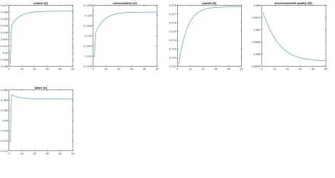
Figures 1 to 3 show how the DCE reacts to a (i) 1% increase in the weight on

remains unchanged), (ii) 1% increase in the weight on environmental quality with a

si-multaneous 1% decrease in the weight on labor-leisure (consumption remains unchanged),

and (iii) 1% increase in the weight on consumption with a simultaneous 1% decrease in

labor-leisure (environmental awareness remains unchanged).

We find that an increase in the weight on environmental quality (environmental

aware-ness) with a relative decrease in the weight on consumption (leisure-labor decision),

keep-ing the third weight steady, leads to a higher (lower) environmental quality and lower

(higher) output (Figures 1 and 2, respectively). In the case where we change the weights

on consumption and leisure-labor decision in opposite directions, all endogenous variables

increase except from environmental quality and welfare. Given these baseline findings,

we move to the optimal tax problem, where the economy moves to a better state given

policy action.

5. Optimal tax with an environmental externality

There are many competitive equilibria indexed by different government policies and

the planner’s problem is to choose the one that maximizes

∞

X

t=0

βt[(ct)µ1(1−nt)µ2(Qt)1−µ1−µ2]1−σ

1−σ ,

subject to the DCE. Therefore, the planner chooses the best competitive equilibrium,

taking as given {gt}∞t=0, k0, Q0, and bounds on taxes, i.e. 0 ≤ τtk < 1 and 0 ≤ τtl < 1.

Moreover, the period zero tax rates, 0 ≤ τk

0 <1 and 0 ≤ τ0l <1 are also taken as given,

otherwise the government would be able to impose lump-sum taxes, which would make

the policy problem first-best.

Optimal taxation provides a compelling argument against taxing capital income in

rt and wt with net factor prices ert and wet, where

e

rt= (1−τtk)rt, (29)

e

wt= (1−τtl)wt. (30)

In this way, the four instruments τk

t, τtl, rt, wt reduce to two.7 Thus, the DCE is given by

ct

1−nt

= µ1

µ2 e

wt, (31)

Uct =βUct+1(ret+1+ 1−δ

k

), (32)

Qt+1 = (1−δq) ¯Q+δqQt−φAktan1t−a+νg, (33)

g =Aka tn

1−a

t −wetnt−ertkt, (34)

ct+kt+1−(1−δk)kt+g =Aktan1− a

t . (35)

The planner’s problem in Langrangian form becomes

L =

∞

X

t=0

βt{U(ct, nt, Qt)

+λt(

µ1

µ2 e

wt−

ct

1−nt

)

+ψt[βUct+1[ert+1+ 1−δ

k_]−U ct]

+ζt[(1−δq) ¯Q+δqQt−ϕAkatn1− a

t +νg−Qt+1]

+ξt(Aktan1− a

t −wetnt+ertkt−g)

+χt[Akatn

1−a

t −ct−kt+1+ (1−δk)kt−g]},

where{λt, ψt, ζt, ξt, χt}∞t=0are sequences of Langrange multipliers (or the the shadow prices

associated with the household’s first order condition with respect to capital), the Euler

equation, government budget constraint, household budget constraint, and law of motion

of environmental quality, respectively. The FOCs of this problem with respect to ct, nt, 7

Qt+1, kt+1, ˜rt, ˜wt, λt, ψt,ζt, ξt, and χt are

Uct =

1 1−nt

λt+χt−∂Uct/∂ct[ψt−1(ert+ 1−δ)−ψt], (36)

Unt =

ct

(1−nt)2

λt−(1−a)Aktan

1−a

t (ξt−ζtφ+χt) (37)

+ξtwet+∂(Uct/µ1)/∂nt[ψt−ψt−1(ert+ 1−δ)],

UQt[ψt(ert+1+ 1−δ

k

)−ψt+1] =

ζt

β −UQt+1−ζt+1δ

q

, (38)

χt=β[χt+1(fkt+1 + 1−δ

k

) +ξt+1(fkt+1−ret+1)−ζt+1φfk], (39)

ξtkt=ψt−1Uct, (40)

λt

µ1

µ2

=ξtnt, (41)

µ1

µ2 e

wt=

ct

(1−nt)

, (42)

Uct =βUct+1[ret+1+ 1−δ

k_{], (43)}

Qt+1 = (1−δq) ¯Q+δqQt−φAktan

1−a

t +νgt, (44)

Aka tn

1−a

t −wetnt−retkt=gt, (45)

ct+kt+1 =Aktan

1−a

t + (1−δ k_)k

t−gt. (46)

Some considerations are in order. Eq. (39), the Euler equation, tells us that a marginal

increase of capital investment in periodtincreases the amount of available goods in period

t+ 1 by (fk+ 1−δ), with social marginal valueχt+1. Moreover, tax revenues increase by

(fk−ert+1), which enables the government to reduce its debt on other taxes by the same

amount. This increase has a social marginal value equal to ξt+1, which is interpreted as

the extra burden imposed to the society due to the existence of distortionary taxation. β

is the discount factor in periodt+ 1 andχt is the social marginal value of the investment

investment worsens environmental quality by φfk, with social marginal value ζt+1.

We obtain the long-run conditions by dropping the time subscripts. To simplify the

FOCs, we set σ= 1 in the utility function U(ct, lt, Qt), which then limits to

U(ct, lt, Qt) =µ1ln(ct) +µ2ln(lt) + (1−µ1−µ2) ln(Qt). (47)

As we did with the DCE, we linearize the system of Eqs. (36)-(46) around the steady state

using Taylor’s Theorem. We use the same values for the parameters and we find that the

model is stable (for details see Appendix B). Once again, there is a unique equilibrium

and the economy converges to this through a saddle path.

5.1. The Chamley-Judd approach to the planner’s problem

Eq. (39) reduces in the long run to

β[(r−_er)ξ+ (r+ 1−δ)χ−rφζ] =χ. (48)

From Eq. (43), it holds in the long run that (1−δ) = 1_β−er. By replacing this result into (48) and rearranging we have

(r−_er)(χ+ξ)−rφζ = 0. (49)

We now consider two cases, where φ= 0 and φ 6= 0. In the first case, the environmental externality is zero and Eq. (49) becomes

τk_{(χ+ξ) = 0. (50)}

The marginal social value of goods χ is strictly positive and the marginal social value of reducing government taxes ξ is nonnegative; therefore, r must equal to r_e, so that τk _is

equal to zero. This is the result of the papers by Chamley (1986) and Judd (1985).

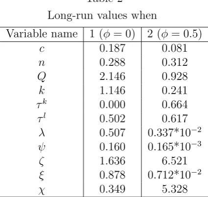
parameter values (same as in the DCE shocks) and in Column 1 of Table 2 the results.

The findings show that τk _{= 0 and the discounted welfare fort= 100 is}

U∗(c, n, Q) = (1−β

t₎

(1−β)U(c, n, Q) =

(1−β100₎

(1−β)

(cµ1(1−n)µ2Q(1−µ1−µ2))(1−σ)

(1−σ) =−53.76943282

In the case, where φ 6= 0, the first term of Eq. (49) is exactly the same with the Chamley-Judd result. The second term of Eq. (49) appears because of the positive

environmental externality. By substituting _erwith r(1−τk_{) and by rearranging the terms}

we have that

τk₌ φζ

χ+ξ, (51)

which is always positive. It must hold that τk _<1⇔ φζ

χ+ξ <1, or φζ < χ+ξ.

8

In Column 2 of Table 2 we provide the results from the numerical example where φ

is positive and equal to 0.5. The values of the parameters are as before. Evidently, τk _is

positive and discounted welfare in this case for t= 100 is given by

U∗(c, n, Q) = (1−β

t₎

(1−β)U(c, n, Q) =

(1−β100₎

(1−β)

(cµ1(1−n)µ2Q(1−µ1−µ2))(1−σ)

(1−σ) =−86.12491269,

The presence of the environmental externality worsens environmental quality. Taxes

in-crease and this leads to a lower level of utility, compared to the case where the

environ-mental externality is equal to zero.

In our model with an environmental externality, taxing capital constitutes a way for the

government to extract revenues generated by a polluting activity and use these revenues

for abatement policy to improve the public good, i.e. the environmental quality. Thus,

we obtain a second-order Chamley-Judd result, where the capital tax is always positive.

8

5.2. Impulse response functions and stylized facts

In this section, we illustrate the dynamic response of the economy to permanent

uni-tary increases in certain parameters of our model. We begin by the equivalent shocks to

the ones we present for the DCE in Section 4.3. Moreover, we study the responses due

to a 1% increase in the weight on the pollution parameter φ and a 1% increase in the abatement technology ν.

Figure 4 shows how the economy responds to a 1% increase in environmental awareness

with a simultaneous 1% decrease in the weight on consumption. We observe that, in the

long-run, output, consumption, and labor decrease. Therefore, there is a channel of

substitution running from consumption to environmental quality. Further, to finance the

exogenous government spending, there is an increase in the labor tax.

In turn, Figure 5 shows how the economy responds to a 1% increase in environmental

awareness with a simultaneous 1% decrease in the weight on labor-leisure. We observe

that, in the long-run, consumption falls and labor increases. Importantly, and in contrast

with Figure 4, capital and output increase along with environmental quality.

Two main results become apparent from these exercises. First, as expected, an increase

in the households’ environmental awareness always leads to a higher environmental quality,

reflecting on the actions of the government. Second, comparing inferences from Figures 4

and 5, we note (as in the DCE) that the substitution between environmental awareness and

consumption lowers output (Figure 4), whereas the substitution between environmental

awareness and labor increases output (Figure 5). In other words, the economy is better

off when the rising environmental awareness goes as far as mitigating households labor

supply toward polluting activities and related jobs. This provides further evidence that

endogenizing labor decisions is important to study the effect of environmental awareness

on households’ decisions and real economic outcomes. Our results are in line with the

empirical findings of Iosifidi (2016), who shows that the environmental awareness-labor

supply nexus is stronger compared to the environmental awareness-consumption nexus.

An interesting issue related to environmental awareness is the case in which this leads

param-eter implies that public abatement spending is transformed more effectively into units

of renewable resources. Based on the results presented in Figure 6, households consume

more, but labor remains approximately constant. The production of the polluting output

increases, but the improvement of abatement technology completely offsets this negative

effect, without raising the capital tax. Environmental quality increases and the economy

moves to a higher-welfare steady state.

6. Conclusions

This paper studies a dynamic general equilibrium model with an environmental

exter-nality and optimal taxation. In our model the households decide between consumption,

labor, and environmental quality. Thus, there are two channels of substitution for

environ-mental quality: that of consumption (as in previous literature) and that of labor-leisure.

We posit that this distinction is important given empirical facts showing a strong effect

of environmental awareness on labor supply.

Our model predicts that an increase in households’ environmental awareness improves

environmental quality and the same also holds when environmental awareness remains

constant and the weight on consumption increases at the expense of the weight on labor.

Importantly, an increase in environmental awareness yields lower output when it is

ac-companied by a decrease in the weight on consumption, ceteris paribus. In contrast, an

increase in environmental awareness has the exact opposite effect on output when it is

accompanied by a decrease in the weight on labor,ceteris paribus. Phrased differently, an

increase in environmental awareness can have both positive or negative effects on output

based on whether it trades off labor (positive effect) or consumption (negative effect).

This finding is consistent with recent evidence on the effect of environmental awareness

on labor supply and related government actions to improve environmental quality via

lower polluting units (and jobs).

We also find that the optimal capital tax in the long run is non-zero. This happens

generated by a polluting activity and use these revenues for abatement policy to improve

environmental quality. As pollution decreases, the government reduces the capital tax

rate to extract a smaller fraction of the rents. When the pollution externality is zero, the

model is equivalent to the standard model of optimal dynamic taxation. In that case,

there are no capital rents produced by polluting activities, so the optimal steady-state

capital tax rate is zero. Thus, our model yields a second-order Chamley-Judd result,

where the capital tax is always positive.

References

Acemoglu, D., Golosov, M., Tsyvinski, A., 2011. Political economy of Ramsey

taxa-tion. Journal of Public Economics 95, 467-475.

Angelopoulos, K., Economides, G., Philippopoulos, A., 2013. First-and second- best

allocations under economic and environmental uncertainty. International Tax and Public

Finance 20, 360-380.

Aznar, R.M., Ruiz-Tamarit, J.R., 2005. Renewable natural resources and endogenous

growth. Macroeconomic Dynamics 9, 170-197.

BBC, 2011. Germany: Nuclear power plants to close by 2022. Available at: http://www.bbc.co.uk/news/w

europe-13592208.

Beltratti, A., 1996. Sustainability and growth: Reflections on economic models.

Kluwer Academic, Dordrecht.

Bernauer, T., Koubi, V., 2009. Political determinants of environmental quality.

Eco-logical Economics 68, 1355-1365.

Bilbiie, F.O., Ghironi, F., Melitz, M.J., 2012. Endogenous entry, product variety, and

business cycles. Journal of Political Economy 120, 304-345.

Bovenberg, A., Smulders, S., 1995. Environmental quality and pollution- 21

augment-ing technological change in a two-sector endogenous growth model. Journal of Public

Economics 57, 369-391.

Resources, edited by Smith, V.L., 441-461, Gordon & Breach, New York.

Chamley, C., 1986. Optimal taxation of capital income in general equilibrium with

infinite lives. Econometrica 54, 607-622.

Correia, I.H., 1996. Should capital income be taxed in the steady state? Journal of

Public Economics 60, 147-151.

Debortoli, D., Gomes, P., 2012. Labor and profit taxation, and the supply of public

capital. Available at: https://ideas.repec.org/p/red/sed012/325.html

De Hek, P.A., 2006. On taxation in a two-sector endogenous growth model with

endogenous labor supply. Journal of Economic Dynamics and Control 30, 655-685.

Dioikitopoulos, V.E., Kalyvitis, S., Vella, E., 2015. Green spending reforms, growth

and welfare with endogenous subjective discounting. Macroeconomic Dynamics 19,

1240-1260.

Economides. G., Philippopoulos A., 2008. Growth enhancing policy is the means to

sustain the environment. Review of Economic Dynamics 11, 207-219.

Economides, G., Pilippopoulos, A., Vasilatos, E., 2008. The primal versus the dual

ap-proach to the optimal Ramsey tax problem. Available at: http://www2.aueb.gr/users/gecon/Economides%20et%20al.%20(June%2018%202007).p

Flores, N.E., Graves, P.E., 2008. Optimal public goods provision: Implications of

endogenizing the labor/leisure choice. Land Economics 84, 701-707.

Fowlie, M., 2009. Incomplete environmental regulation, imperfect competition, and

emissions leakage. Economic Policy 1, 72-112.

Iosifidi, M., 2016. Environmental awareness, consumption, and labor supply:

Empiri-cal evidence from household survey data. EcologiEmpiri-cal Economics 129, 1-11.

John, A., Pecchenino, R., 1994. An overlapping generations model of growth and the

environment. Economic Journal 104, 1393-1410.

Jones, L.E., Manuelli, R.E., Rossi, P.E., 1997. On the optimal taxation of capital

income. Journal of Economic Theory 73, 93-117.

Jouvet, P.A., Philippe, M., Gilles, R., 2005. Optimal growth with pollution: How to

use pollution permits? Journal of Economic Dynamics and Control 29, 1597-1609.

of Public Economics 28, 59-83.

King, R.G., Rebelo, S.T., 1999. Resuscitating real business cycles. Handbook of

Macroeconomics, edited by Taylor, J.B., Woodford, M., chapter 14, pp. 927-1007,

Else-vier.

Kydland, F.E., Prescott, E.C., 1982. Time to build and aggregate fluctuations.

Econo-metrica 50, 1345-1370.

Ljungqvist, L., Sargent, T.J., 2004. Recursive macroeconomic theory. Second Edition,

MIT Press.

Plosser, C.I., 1989. Understanding real business cycles. Journal of Economic

Perspec-tives 3, 51-77.

Smulders, S., 2000. Economic growth and environmental quality. Principles of

Evi-ronmental Econmics, edited by Folmer, H., Gabel, L., Edward Elgar, Cheltenham.

Special Eurobarometer 468, 2017. Attitudes of European citizens towards the

envi-ronment. Available at: http://ec.europa.eu/environment/eurobarometers en.htm.

Stiglitz, J.E., 1987. Pareto efficient and optimal taxation and the new welfare

eco-nomics. Handbook of Public Economics, edited by Auerbach, A.J., Feldstein, M., volume

2, chapter 15, 991-1042.

Turnovsky, S.J., 2000. Fiscal policy, elastic labor supply, and endogenous growth.

Journal of Monetary Economics 45,185-210.

Xepapadeas, A., 2005. Economic growth and the environment. Handbook of

Table 1

Parameter values for the numerical example

Parameter Description Value

a Capital share in production 0.33

δk _{Capital depreciation rate 0.1}

σ Curvature parameter in utility function 2

β Time discount factor 0.97

µ1 Consumption weight in utility function 0.3

µ2 Leisure weight in the utility function 0.3

¯

Q Environmental quality without pollution 1

δq _{Persistence of environmental quality 0.9}

A Long-run total factor productivity 1

φ Long-run pollution externality 0.5

ν Transformation of spending into units of nature 0.75

Table 2

Long-run values when

Variable name 1 (φ= 0) 2 (φ = 0.5)

c 0.187 0.081

n 0.288 0.312

Q 2.146 0.928

k 1.146 0.241

τk _{0.000 0.664}

τl _{0.502 0.617}

λ 0.507 0.337*10−2

ψ 0.160 0.165*10−3

ζ 1.636 6.521

ξ 0.878 0.712*10−2

Figure 1: Response of the DCE with endogenous labor to an increase in µ3, decrease in

µ1, with steady µ2

0 20 40 60 80 0.43 0.431 0.432 0.433 0.434 0.435 0.436 0.437 0.438

0.439 output (y)

0 20 40 60 80 0.1215

0.122 0.1225 0.123 0.1235

0.124 consumption (c)

0 20 40 60 80 0.364 0.365 0.366 0.367 0.368 0.369 0.37 0.371

0.372 capital (k)

0 20 40 60 80 0.8875

0.888 0.8885 0.889 0.8895

0.89 environmental quality (Q)

0 20 40 60 80 0.466 0.467 0.468 0.469 0.47 0.471 0.472 0.473 0.474 0.475

0.476 labor (n)

Figure 2: Response of the DCE with endogenous labor to an increase in µ3, decrease in

µ2, with steady µ1

0 10 20 30 40 50 0.438 0.439 0.44 0.441 0.442 0.443 0.444 0.445 0.446

0.447 output (y)

0 10 20 30 40 50 0.1235 0.124 0.1245 0.125 0.1255 0.126

0.1265 consumption (c)

0 10 20 30 40 50 0.371 0.372 0.373 0.374 0.375 0.376 0.377

0.378 capital (k)

0 10 20 30 40 50 0.8855

0.886 0.8865 0.887 0.8875

0.888 environmental quality (Q)

0 10 20 30 40 50 0.474 0.476 0.478 0.48 0.482 0.484

Figure 3: Response of the DCE with endogenous labor to an increase in µ1, decrease in

µ2, with steady µ3

0 10 20 30 40 50 0.438 0.44 0.442 0.444 0.446 0.448 0.45 0.452

0.454 output (y)

0 10 20 30 40 50 0.1235 0.124 0.1245 0.125 0.1255 0.126 0.1265 0.127 0.1275 0.128

0.1285 consumption (c)

0 10 20 30 40 50 0.37

0.375 0.38

0.385 capital (k)

0 10 20 30 40 50 0.8835 0.884 0.8845 0.885 0.8855 0.886 0.8865 0.887 0.8875

0.888 environmental quality (Q)

0 10 20 30 40 50 0.474 0.476 0.478 0.48 0.482 0.484 0.486 0.488 0.49 0.492

0.494 labor (n)

Figure 4: Response of the economy to an increase in µ3, decrease inµ1, with steady µ2

0 20 40 60 80 0.426 0.428 0.43 0.432 0.434 0.436

0.438 output (y)

0 20 40 60 80 0.115 0.1155 0.116 0.1165 0.117 0.1175 0.118 0.1185 0.119 0.1195

0.12 consumption (c)

0 20 40 60 80 0.466 0.468 0.47 0.472 0.474 0.476

0.478 labor (n)

0 20 40 60 80 0.35 0.352 0.354 0.356 0.358 0.36 0.362 0.364 0.366

0.368 capital (k)

0 20 40 60 80 0.916 0.918 0.92 0.922 0.924 0.926 0.928 0.93 0.932 0.934

0.936 environmental quality (Q)

0 20 40 60 80 0.624 0.626 0.628 0.63 0.632 0.634 0.636

0.638 labor tax

0 20 40 60 80 0.66 0.68 0.7 0.72 0.74 0.76 0.78 0.8

Figure 5: Response of the economy to an increase in µ3, decrease inµ2, with steady µ1

0 10 20 30 40 50 60 0.436 0.438 0.44 0.442 0.444 0.446

0.448 output (y)

0 10 20 30 40 50 60 0.1191 0.1192 0.1193 0.1194 0.1195 0.1196 0.1197 0.1198 0.1199 0.12

0.1201 consumption (c)

0 10 20 30 40 50 60 0.474 0.476 0.478 0.48 0.482 0.484 0.486 0.488 0.49

0.492 labor (n)

0 10 20 30 40 50 60 0.36 0.362 0.364 0.366 0.368 0.37 0.372

0.374 capital (k)

0 10 20 30 40 50 60 0.916 0.918 0.92 0.922 0.924 0.926 0.928 0.93 0.932 0.934

0.936 environmental quality (Q)

0 10 20 30 40 50 60 0.624 0.626 0.628 0.63 0.632 0.634 0.636

0.638 labor tax

0 10 20 30 40 50 60 0.66 0.67 0.68 0.69 0.7 0.71 0.72 0.73

0.74 capital tax

Figure 6: Response of the economy to 1% increase in the abatement technology

0 20 40 60 80 0.436 0.437 0.438 0.439 0.44 0.441

0.442 output (y)

0 20 40 60 80 0.1198 0.12 0.1202 0.1204 0.1206 0.1208 0.121 0.1212 0.1214 0.1216

0.1218 consumption (c)

0 20 40 60 80 0.474 0.475 0.476 0.477 0.478 0.479 0.48 0.481 0.482 0.483

0.484 labor (n)

0 20 40 60 80 0.364 0.366 0.368 0.37 0.372 0.374 0.376 0.378 0.38

0.382 capital (k)

0 20 40 60 80 0.915

0.92 0.925 0.93 0.935

0.94 environmental quality (Q)

0 20 40 60 80 0.614 0.616 0.618 0.62 0.622 0.624 0.626 0.628

0.63 labor tax

0 20 40 60 80 0.65 0.66 0.67 0.68 0.69 0.7

Appendix A: Linearization of the DCE

Eq. (26) becomes

f(ct, kt+1, kt, nt) = ˆct+ ˆkt+1+faˆnt+fbˆkt= 0, (A1)

where for any variable xof the system it holds that ˆxt=xt−x∗, withx∗ being the steady

state value of the variable and

fa=fnt(·) = [−A(1−a)(k

∗₎a_(n∗₎−a_[1−aτk_−(1−a)τl_{]], (A2)}

fb =fkt(·) = [−[aA(k

∗₎a−1_(n∗₎1−a_[1−aτk_−(1−a)τl_{] + (1−δ}k_{)]]. (A3)}

Eq. (27) becomes

g(ct, kt, nt) =µ2ˆct+ganˆt+gbkˆt = 0, (A4)

where

ga =gnt(·) = [µ1aA(k

∗₎a_(n∗₎−a−1_+µ

1(1−a)A(k∗)a(n∗)−a](1−τl)(1−a), (A5)

gb =gkt(·) = [−µ1(1−n

∗_)(1−a)aA(k∗₎a−1_(n∗₎−a

(1−τl)]. (A6)

Eq. (28) becomes

h(ct+1, nt+1, Qt+1, kt+1, ct, nt, Qt) =haˆct+1+hbnˆt+1+hcQˆt+1 (A7)

where

ha=hct+1(·) = −[β[µ1(1−σ)−1](c

∗₎µ1(1−σ)−2_[(1−n∗₎µ2_(Q∗₎1−µ1−µ2_]1−σ_{] (A8)}

[(1−τk)aA(k∗)a−1(n∗)1−a+ 1−δk], hb =hnt+1(·) = [βµ2(1−σ)(c

∗₎µ1(1−σ)−1_(1−n∗₎µ2(1−σ)−1_(Q∗₎(1−µ1−µ2)(1−σ) _(A9)

[(1−τk_)aA(k∗₎a−1_(n∗₎1−a_{+ 1−δ}k_{]−β(1−a)(c}∗₎µ1(1−σ)−1

[(1−n∗)µ2

(Q∗)1−µ1−µ2

]1−σ[(1−τk)aA(k∗)a−1(n∗)−a], hc =hQt+1(·) = −[β(1−µ1−µ2)(1−σ)(c

∗₎µ1(1−σ)−1 _(A10)

(1−n∗)µ2(1−σ)_(Q∗₎(1−µ1−µ2)(1−σ)−1_][(1−τk_)aA(k∗₎a−1_(n∗₎1−a_{+ 1−δ}k_],

hd=hkt+1(·) = [−β(c

∗₎µ1(1−σ)−1

(1−n∗)µ2(1−σ)

(Q∗)(1−µ1−µ2)(1−σ)

(A11)

(1−τk_)a(a−1)A(k∗₎a−2_(n∗₎1−a_],

he =hct(·) = [[µ1(1−σ)−1](c

∗₎µ1(1−σ)−2_[(1−n∗₎µ2_(Q∗₎1−µ1−µ2_]1−σ_{, (A12)}

hf =hnt(·) =−[µ2(1−σ)(c

∗₎µ1(1−σ)−1_(1−n∗₎µ2(1−σ)−1_(Q∗₎(1−µ1−µ2)(1−σ)_{], (A13)}

hg =hQt(·) = [(1−µ1−µ2)(1−σ)(c

∗₎µ1(1−σ)−1_(1−n∗₎µ2(1−σ)_(Q∗₎(1−µ1−µ2)(1−σ)−1_].

(A14)

Finally Eq. (29) becomes

m(Qt+1, nt, Qt, kt) = δqQˆt+maˆnt+mbˆkt−Qˆt+1 = 0, (A15)

where

ma =mnt(·) = −A(1−a)(k

∗₎a_(n∗₎−a_[v[aτk_{+ (1−a)τ}l_{]−φ], (A16)}

mb =mkt(·) =−aA(k

∗₎a−1_(n∗₎1−a_[v[aτk_{+ (1−a)τ}l_{]−φ]. (A17)}

        

0 0 −1 0

0 0 0 0

−ha −hb −hd −hc

0 0 0 1

                  ˆ

ct+1

ˆ

nt+1

ˆ

kt+1

ˆ

Qt+1

         =         

fa 1 fb 0

µ2 ga gb 0

hf he 0 hg

ma 0 mb δq

                  ˆ ct ˆ nt ˆ kt ˆ Qt         

⇐⇒ AXˆt+1 =

BXˆt.

One way to check the stability of equilibrium is with the approach of Blanchard and

Kahn (1980). We observe that the second equation is a static equation. We substitute

this equation into the other three equations of the system and the system becomes      

0 1 0

h1 h2 hc

0 0 1             ˆ

ct+1

ˆ

kt+1

ˆ

Qt+1

     =      

f1 f2 0

h3 h4 −hg

m1 m2 δq

            ˆ ct ˆ kt ˆ Qt      ⇔E

ˆ

Xt+1 =FXˆt ⇔Xˆt+1 =F E−1Xˆt⇔

ˆ

Xt+1 =CXˆt.

Using the parameter values in the paper of Angelopoulos, Economides, and

Philip-popoulos (2013), we find that there are two eigenvalues with module smaller than 1 for

the backward looking variables ˆkt and ˆQt, and one eigenvalue with module larger than 1

for the forward looking variable ˆct. When we solve the 4 by 4 system using Dynare we

find that the eigenvalue of nt, which is a forward looking variable too, has module larger

than 1. The Blanchard-Kahn conditions are satisfied and the model is stable. The steady

state of the system is a saddle path, therefore it has a unique equilibrium.

Given that in the initial 4 by 4 system the matrix A is singular, we can also check its stability using the approach of Klein (2000). We first recover the generalized Schur

decomposition of (A, B). We get the matrices of complex numbers Q and Z, such that

S =QAZ and T =QBZ are upper triangular, and QQ′ _=ZZ′ _{=I. Then the dynamics}

equation can be rewritten as

AZZ′Xt+1 =BZZ′Xt. (A18)

Let us define ̟t =Z′Xt to get

and pre-multiply both sides by Q

QAZ̟t+1 =QBZ̟t, (A20)

which is equal to

S̟t+1 =T ̟t. (A21)

Tii

Sii are the generalized eigenvalues of the system. We find that we have two stable

eigen-values with modulus below unity, which are associated with the variables kt and Qt, and

two unstable eigenvalues with modulus greater than unity, which are associated with the

variables ct and nt. Therefore, the model is stable, the steady state of the system is a

saddle path and it has a unique equilibrium.

Appendix B: Linearization of the optimal tax model

For

the FOCs of the Ramsey problem become:

µ1ct−

c2

tλt

1−nt

+βψt

µ1

c2

t

−c2_tχt−ψt−1

µ1

c2

t

[(1−τk t)Ak

a tn

1−a

t + 1−δ

k_{] = 0, (B2)}

(1−a)Akatn− a

t [χt−ζtφ+ξt[aτtk+ (1−a)τ l

t]] (B3)

+ψt−1

µ1

ct

(1−τl

t)a(1−a)Ak a−1

t n

−a t

− ctλt

(1−nt)2

−λt(1−τtl)

µ1

µ2

a(1−a)Aka tn

−1−a t = 0,

ψt

µ1

ct+1

(1−τk

t+1)a(a−1)Akta+1−2n1t+1−a−

χt

β +λt+1(1−τ

l t+1)

µ1

µ2

a(1−a)Aka−1

t+1n−t+1a (B4)

+aAka−1

t+1n1t+1−a(χt+1−ζt+1φ+ξt+1[aτtk+1+ (1−a)τtl+1]) +χt+1(1−δk) = 0, −ζtQt+1+β(

1−µ1−µ2

Qt+1

+ζt+1δq) = 0, (B5)

ξtkt−ψt−1

µ1

ct

= 0, (B6)

ξtnt−λt

µ1

µ2

= 0, (B7)

µ1

µ2

(1−a)Aka

tn−ta(1−τtl)−

ct

1−nt

= 0, (B8)

β µ1 ct+1

[(1−τtk+1)aAk

a−1

t+1n1−

a

t+1 + 1−δ

k

] = µ1

ct

, (B9)

Qt+1 = (1−δq) ¯Q+δqQt−φAktan

1−a

t +νg, (B10)

g =Aka tn1−

a t [aτ

k

t + (1−a)τ l

t], (B11)

ct+kt+1 =Akatn1− a

t −g+ (1−δ k

)kt. (B12)

(B5) and (B6) at time t and t+ 1, so that Eqs. (B2)−(B12) be written as

µ1ct−

c2

tλt

1−nt

+βξt+1kt+1ct+1−c2tχt−ξtktct[(1−τtk)Ak a tn

1−a

t + 1−δ

k_{] = 0, (B13)}

(1−a)Aka tn

−a

t [χt(1−

ϕ

ν) +ξt[aτ

k

t + (1−a)τ l t−

ϕ ν]]−

µ2

1−nt

+ξt(1−τtl)a(1−a)Ak a tn

−a t

(B14)

− ctλt

(1−nt)2

−λt(1−τtl)

µ1

µ2

a(1−a)Aktan−1− a t = 0,

ξt+1kt+1(1−τtk+1)a(a−1)Ak

a−2

t+1n1−

a t+1 −

χt

β +λt+1(1−τ

l t+1)

µ1

µ2

a(1−a)Akat+1−1n−

a

t+1 (B15)

+aAkat+1−1nt1+1−a[χt+1(1−

ϕ

ν) +ξt+1[aτ

k

t+1+ (1−a)τtl+1−

ϕ

ν]] +χt+1(1−δ

k

) = 0,

−(χt+ξt)

1

νQt+1+β

1−µ1−µ2

Qt+1

+ βδ

q

ν (χt+1+ξt+1) = 0, (B16) ξtnt−λt

µ1

µ2

= 0, (B17)

µ2ct−µ1(1−nt)(1−a)Akatn

−a t (1−τ

l

t) = 0, (B18)

βµ1ct[(1−τtk+1)aAkat+1−1n1t+1−a+ 1−δk] =µ1ct+1, (B19)

(1−δq) ¯Q+δqQt−ϕAktan1− a

t +νAk a tn1−

a t [aτ

k

t + (1−a)τ l

t]−Qt+1 = 0, (B20)

ct+kt+1−Akatn

1−a

t [1−aτ k

t −(1−a)τ l

t]−(1−δ k_)k

t= 0. (B21)

In this way we have a system with nine equations in{ct, nt, kt+1, Qt+1, τtk, τtl, λt, χt, ξt}∞t=0.

We linearize Eqs. (B13)−(B21) around the steady state to analyze the system’s behav-ior. By using Taylor’s theorem we expand the functions of the system around the steady

state.

Eq. (B13) becomes

f1(ct, nt, λt, ξt+1, kt+1, ct+1, χt, ξt, kt, τtk) =f1acˆt+f1bnˆt+f1cλˆt+f1dξˆt+1+f1eˆkt+1 (B22)

where

f1a =f1ct(c

∗_{, n}∗_{, λ}∗_{, ξ}∗_{, k}∗_{, c}∗_{, χ}∗_{, ξ}∗_{, k}∗_{, τ}k∗_{) = [µ}

1−

2c∗_λ∗

1−n∗ −2c

∗_χ∗_−ξ∗_k∗_[(1−τk∗₎

(B23)

A(k∗)a(n∗)1−a+ 1−δk]], f1b =f1nt(c

∗_{, n}∗_{, λ}∗_{, ξ}∗_{, k}∗_{, c}∗_{, χ}∗_{, ξ}∗_{, k}∗_{, τ}k∗_{) = [−[} (c∗)2λ∗

(1−n∗₎2 (B24)

+ξ∗k∗c∗(1−τk∗)(1−a)A(k∗)a(n∗)−a]], f1c =f1λt(·) = [−

(c∗₎2

1−n∗], (B25)

f1d=f1ξt+1(·) =βk

∗_c∗_{, (B26)}

f1e =f1kt+1(·) = βξ

∗_c∗_{, (B27)}

f1f =f1ct+1(·) = βξ

∗_k∗_{, (B28)}

f1g =f1χt(·) = [−(c

∗₎2_{], (B29)}

f1h =f1ξt(·) = [−[k

∗_c∗_[(1−τk∗_)A(k∗₎a

(n∗)1−a+ 1−δk]]], (B30)

f1i =f1kt(·) = [−ξ

∗_c∗_[(1−τk∗_)A(k∗₎a_(n∗₎1−a_{+ 1−δ}k_{] (B31)}

−ξ∗c∗(1−τk∗)Aa(k∗)a(n∗)1−a], f1j =f1τk

t(·) =ξ

∗_c∗_(1−τk∗_)A(k∗₎a+1_(n∗₎1−a

. (B32)

Eq. (B14) becomes

f2(kt, nt, χt, ξt, τtk, τtl, ct, λt) =f2aˆkt+f2bnˆt+f2cχˆt+f2dξˆt+f2eτˆtk+f2fτˆtl+f2gcˆt+f2hλˆt,

where

f2a =f2kt(·) = [(1−a)aA(k

∗₎a−1_(n∗₎−a_[χ∗₍₁₋ φ

ν) (B34)

+ξ∗[aτk∗+ (1−a)τl∗− φ

ν]] +ξ

∗_(1−τl∗_)a2_(1−a)A(k∗₎a−1_(n∗₎−a

−λ∗(1−τl∗₎µ1

µ2

a2(1−a)A(k∗)a−1_(n∗₎−1−a_],

f2b =f2nt(·) = [−a(1−a)A(k

∗₎a_(n∗₎−a−1_[χ∗₍₁₋ φ

ν) (B35)

+ξ∗[aτk∗_{+ (1−a)τ}l∗ ₋φ

ν]]− µ2

(1−n∗₎2 −ξ

∗_(1−τl∗_)a2_(1−a)A(k∗₎a_(n∗₎−a−1

−2c

∗_λ∗_(1−n∗₎

(1−n∗₎4 +λ

∗_(1−τl∗₎µ1

µ2

a(1−a)(a+ 1)A(k∗)a(n∗)−a−2],

f2c =f2χt(·) = (1−a)A(k

∗₎a

(n∗)−a(1− φ

ν), (B36) f2d=f2ξt(·) = [(1−a)A(k

∗₎a_(n∗₎−a_{, (B37)}

[aτk∗_{+ (1−a)τ}l∗₋ φ

ν]] + (1−τ

l∗_)a(1−a)A(k∗₎a_(n∗₎−a_{], (B38)}

f2e =f2τk

t(·) = (1−a)A(k

∗₎a

(n∗)−aξ∗a, (B39)

f2f =f2τl

t(·) = [(1−a)

2_A(k∗₎a_(n∗₎−a_ξ∗_−ξ∗_a(1−a)A(k∗₎a_(n∗₎−a _(B40)

+λ∗µ1 µ2

a(1−a)A(k∗)a_(n∗₎−a−1_],

f2g =f2ct(·) = [−

λ∗

(1−n∗₎2], (B41)

f2h =f2λt(·) = [−

c∗

(1−n∗₎2 −(1−τ

l∗₎µ1

µ2

a(1−a)A(k∗)a_(n∗₎−a−1_{]. (B42)}

Eq. (B15) becomes

f3(ξt+1, kt+1, τtk+1, nt+1, χt, λt+1, τtl+1, χt+1) = f3aξˆt+1+f3bkˆt+1+f3cτtk+1+f3dnˆt+1 (B43)