Munich Personal RePEc Archive
Energy consumption, trade openness,
economic growth, carbon dioxide
emissions and electricity consumption:
evidence from South Africa based on
ARDL
Hasson, Ashwaq and Masih, Mansur
INCEIF, Malaysia, INCEIF, Malaysia
13 May 2017
Online at
https://mpra.ub.uni-muenchen.de/79424/
1
Energy consumption, trade openness, economic growth, carbon dioxide emissions
and electricity consumption: evidence from South Africa based on ARDL
Ashwaq Hasson1 and Mansur Masih2
ABSTRACT
This paper undertakes to investigate the interplay between economic growth, energy consumption, electricity consumption, carbon emission and trade by employing recent South African trade and energy data during the period from 1971 to 2013. South Africa is used as a case study given its status as perhaps the most developed country in the African continent with a very high energy consumption as well as its unique position in its current history where it relies on the somewhat antiquated coal industry to provide most of its energy as well as being one of its main imports. The effect of trade openness on environmental conditions has spawned a great deal of controversy in the current energy economics literature. Although research on the relationship between energy consumption, carbon emissions and economic growth are quite prevalent, no study to our knowledge specifically addresses the role that South Africa’s trade plays in this context. The ARDL bounds testing approach to cointegration has been used to test the long run relationship among the variables, while short run dynamics has been investigated by applying error correction method (ECM). The main finding of interest in this paper is that a positive relationship exists between energy consumption and economic growth. However, it seems the results suggest that electricity prices have a negative impact on economic growth. The results further evidenced that trade openness and electricity are leading variables, while the rest are lagging. Furthermore, our results demonstrate trade reduces overall pollutions caused by carbon emission, thus it improves environmental quality by contracting the growth of energy pollutants. Our empirical results are consistent with the existence of environmental Kuznets curve. It is, thus, imperative for policymakers to take better care of these two
exogenous variables that will have a profound effect on the country’s economy as a whole. The policymakers should make decision on GDP based on trade openness because changes in trade openness will have impact on GDP, as trade is a leading variable.
Key words: GDP, Energy consumption, Trade openness, EKC, Carbon Emission, South Africa.
1Graduate student in Islamic finance at INCEIF, Lorong Universiti A, 59100 Kuala Lumpur, Malaysia.
2Corresponding author, Professor of Finance and Econometrics, INCEIF, Lorong Universiti A, 59100 Kuala Lumpur,
2 1.0.Introduction
Although there isn’t any concrete connection given in mainstream economic theories that point to a relationship between energy consumption and economic growth, empirical analysis attempting to prove or disprove this potential relationship has been one of the most pursued
areas of energy economics literature in recent decades. Many studies have investigated the
causal relationship between energy consumption and economic growth. With energy being one
of the most crucial aspects of modern life and as such, its consumption is an essential
component of economic development. To this end, according to economic theory such as the
Jevons Paradox3, an increase in energy consumption ultimately does have an effect on economic growth. As such, energy is crucial for the economies of both developed countries as
well as developing countries, and as mentioned previously, this area of study on the relationship
between energy consumption and economic growth has been heavily focused on by experts as
it is very consequential towards the policies implemented by the policy makers. The
ever-increasing production in the world throughout history has naturally increased the need for
energy. However, the finite nature of oil and natural gas resources in the world poses a threat
overall economic growth.
There has been a continuing discussion over how the existence and use of abundant natural
resources and energy sources affect and are affected by geopolitics and corruption, and how
this can propel or stagnate economic progress. This debate is usually referred to as the
Resource Curse4 which posits that there is a paradox present in countries with an abundance
of non-renewable natural resources, in that they tend to have less economic growth, less
democracy, and worse development than countries with fewer natural resources (Venables
2016). This is theorized to happen for multiple reasons, and there is much debate among
experts over these particulars. Most experts believe that this so-called curse is not in fact
universal or unavoidable, but instead affects only certain types of countries under specific
conditions.
Overall, emerging economies have experienced significant economic growth rates during the
past decades. This paper will focus on the relationship between energy consumption, trade,
3 Jevons, William Stanley, 1865/1965. In: Flux, A.W. (Ed.), The Coal Question: An Inquiry Concerning the Progress of the Nation, and the Probable Exhaustion of Our Coal-mines, 3rd edition 1905. Augustus M. Kelley, New York
4Soros, G. (2007). Escaping the Resource Curse (HUMPHREYS M., SACHS J., & STIGLITZ J.,
3
carbon emission, electricity use and economic growth for one such economy, namely that of
South Africa. South Africa was selected as a case study because it is one of the largest
economies in the economically fast-growing and resource-rich continent of Africa. In fact, it is
the world’s most carbon-intensive non-oil-producing developing country as well as being one
of the 6 largest exporters of coal in the world. Most of South Africa’s liquid fuel requirements are imported in the form of crude oil. Also, South Africa’s per capita energy consumption as
of 2013 is 2655.9 kg oil equivalent, which is much more than the world average of 1680 kg oil
equivalent and has the highest demand for electricity in Africa.
This leaves South Africa in a conundrum however, as their economic growth relies on their
coal production and exportation. How does the African power decrease Greenhouse Gas
emissions without negatively affecting its economy? As such, this paper will investigate that
the nature of the relationship between energy consumption, trade, electricity use, economic
growth and carbon emissions is investigated in order to determine the most suitable policies to
address this conundrum.
South Africa has a high level of energy consumption and a heavy dependence on energy
imports. As such it relies heavily on coal as its main source of energy. This presents multiple
problems; for one, the developed countries have been moving away from coal as an energy
source for many years. In countries such as the United States for example, multiple coal mines
have been shut down as the country moves forward. The complicated by concerns the fact that
price of coal is increasing especially relative to other energy sources. This issue is also
intertwined with the very harmful issue of the Greenhouse Effect which is a by-product of coal
emissions. This leaves South Africa at a very crucial juncture in its history regarding its
economic future.
In addition, South Africa is facing constant power outages between the years 2008 and 2014,
this crisis occurred due to the sudden drop in the electricity supply reserve margins
(Eskom,2014). As a consequence, production levels in major sectors of the economy such as
commercial, mining industries and industrial have decline. Thus, the signal that arise from
these on-going power outages is the consideration of the dissonance between economic growth
4 2.0.Literature Review and Theoretical Bases
One of the primary sources of energy in today is electricity. Electricity is an essential source
of energy and it is effective in taking care of households and industrial consumers (Salehen et al., 2012). It provides a considerable amount of benefit to capital and labor (Ghosh, 2009). It
also boosts international trade5. This is because the supply of electricity is enhanced by technology, and emerging nations are supported to import high technological inputs into
generation from developed nations. As a result, a productive supply of electricity can lead to a
reduction in poverty and expand economic growth. 6. But still it can also be said that economic growth can be improved by boosting electricity consumption.
A collection of studies proved that electricity consumption and economic growth have a long
run relationship (Mozumder and Marathe, 2007; Ahamad et al., 2013; Adebola and Shahbaz,
2013; Masuduzzaman, 2013. The studies confirmed that electricity consumption and economic
growth move together in a long run. Although there is a wealth of scholarship addressing and
analysing the relationship between energy consumption and economic growth, there hasn’t
been a consensus among experts by any measure. Many scholars have found a positive causal
link, take for instance, Khan and Qayyum (2006) who found a positive relationship between
energy consumption and GDP and that energy use played a crucial role in generating and
stimulating economic activity in these nations. However, there were some who even found a
negative link. In fact, there is empirical evidence linking resource abundance with poor
economic growth this was found by Sachs and Warner in 1995. More specifically, over a period
of 33 years from 1965 - 1998, OPEC member nations experienced an average decrease of 1.3%
in per capita gross national product versus an average growth rate of 2.2% in the rest of the
developing world (Gylfason, 2000). This showed that although these countries were wealthy
in terms of natural resources, their economy still suffered on average.
Esso (2010) also noted lack of consensus among scholars about this relationship. He attributes
it to the level of development the country in question has reached, different methodologies used
by the scholars, omitted variable bias and climate conditions among other things. One
inadequacy noted by Fallahi (2011) in the literature is the assumption that energy and economic
5 Samuel, U.P., Lionel, E. (2013), The dynamic analysis of electricity supply and economic development: Lessons from Nigeria. Journal of Sustainable Society, 2(1), 1-11.
5
growth maintain the same relationship over time. Gross (2012) posits that to overcome this
single relationship between energy and growth one must account for structural breaks when
the world experienced, for example, serious crises.
Saad and Belloumi (2015) found in their analysis of the energy consumption, carbon emissions and economic growth of Saudi Arabia that energy price in particular is the most important
variable in explaining economic growth according to the results of the variance composition.
According to them, this result is to be expected, using Saudi Arabia as an example where it is
noted that rises in oil prices contribute significantly to their economic growth. In India,
Mohapatra and Giri (2015) observe that the energy consumption has a positive impact on
economic growth. Their use of the Granger causality test also illuminated the existence of a
bi-directional causal relationship between energy consumption and economic growth in India.
Closer to South Africa, in Nigeria, Akpan & Akpan (2012) observe that their empirical analysis
using the Multivariate Vector Error Correction (VECM) framework returns evidence of
long-run relationship among the variables. However, they found that the EKC hypothesis7 was not
validated by their results. Instead they found that electricity consumption and emissions are
negatively related. This negative could be as a result of the large imbalance between the supply
and demand of electricity in Nigeria. Similarly when it comes South Africa itself, Ben Nasr et
al. (2014) also found no support for the EKC hypothesis.
In a large study of the impact of CO2 emissions and economic growth on energy consumption
encompassing 58 countries, Saidi and Hammami (2015) found a positive and statistically
significant relationship. Similarly, CO2 emissions also have a positive effect on energy
consumption. They conclude that this implies that economic growth, CO2 emissions and
energy consumption are complementary.
Ben Aïssa et al (2014) studied the link amongst GDP, trade, and renewable energy consumption
by employing data of 11 African countries between 1980 and 2008. The long run analysis
results show a bidirectional links between GDP and trade variables and unidirectional
relationship going from renewable energy and trade to GDP. nonetheless, the findings for the
6
short term agree with the bidirectional relationship among trade and GDP and deny the possible
link across GDP and renewable energy and between trade and renewable energy. Antweiler et
al. (2001) analyzed multiple trade measure and demonstrated that that there is in fact a positive
and significant relationship amongst trade openness and growth. Furthermore, economic
theories in international trades postulates that some of the gain and losses is linked with environmental influence of trade. Free trade has beneficial and detrimental effects on
environmental condition. Free trade is beneficial in the sense that it introduces friendly
techniques of production.8 It may be detrimental by moving corrupt industries from wealthy to poor nation. To add, there is positive link among carbon emission and energy consumption.
The measure of trade openness can be separated into two categories. First, measures of trade
volume and second, measures of trade restrictions.
Many reports have theorized that exports are a key element in economic growth
(Vamvoukas, 2007). This confirms with macroeconomic theory since exports are injections to
the economy (Kaldor, 1967; Romer, 1989; Krueger, 1990; Ahmed et al., 2000). The export
sector has also spill-over effects on the production process of the rest of the economy which
leads to a higher total productivity. Furthermore, through a higher degree of specialization, the
country can reap the benefits of economies of scale and comparative advantage. It could be
then said that promoting exports may aid the country to import high value inputs, products and
technologies that may have a positive impact on economy’s overall productive capacity (
Krisna et al., 2003; Vamvoukas, 2007). Therefore, exports eases the biding foreign exchange
constraint and permits increases in productive intermediate imports. They may also accelerate
the adoption of new practices since firms that operate in the world economy are compelled to
remain efficient and competitive by utilizing the latest technological developments in their
production process. In addition, firms have incentives to increase R&D in order to keep up with
foreign competition.
Another study by Arman and Barzegar (2012) studied the impact of trade liberalization on
energy use in a sample of 62 developing countries during 1990-2010. Results show a
meaningful and positive effect of trade liberalization on energy use in these countries. It means
with 1% of increment in trade liberalization, energy use would climb by 0.02%
7
In this paper, we will attempt find out whether energy consumption incites or hinders economic
growth. This paper is not confined to only the nexus between energy consumption and
economic growth, but also extends to trade, electricity use and carbon emissions (pollution) by
employing the autoregressive distributive lag (ARDL) method.
3.0.Data and Methodology
3.1.Data
In this paper, we have taken annual data over the period from 1971 to 2013 (before and
after the oil crisis). The study comprises of time series data on economic growth, energy
consumption, CO2 emissions (metric tons per capita) per capita, trade openness,
electricity consumption and GDP, a proxy for economic growth, of the South African
economy. All the necessary information was extracted from the World Development
Indicators (WDI) published by the World Bank. The figure below tabulates a description
of each variable.
Gross domestic product (GDP) in US$ constant used as proxy for economic growth.
Energy consumption (ENCON) measured in kg of oil equivalent per capita.
Carbon dioxide emission (CO) measured in metric tons per capita is used as proxy
for environmental pollution.
Electricity consumption (EL) is quantified as Kilowatt hours (kWh) per capita,
which measures the production of power plants and combined heat and power plans
less transmission, distribution, and transformation losses and own use by heat and
power plants.
Trade openness (OP) is the sum of exports and imports of goods and services
measured as a share of gross domestic product
4.0. Methodology
In this paper, we employ the ARDL bounds testing cointegration approach created by
Pesaran, Shin, and Smith (2001) to inspect whether a long run dynamic relationship exists
between GDP, energy consumption, trade openness, carbon emission and electricity
8
between variables in numerous studies. Two of these approaches are taken from Engle and
Granger (1987) in the bivariate case and Johansen and Juselius (1990) when multivariate, and
require that all the series should be integrated at the order of integration I(1). The ARDL
bounds testing approach is more appropriate compared to those traditional cointegration
approaches. The approach avoids endogeneity problems and the inability to test long run relationships of variable associates with the traditional Engel-Granger method. Both short run
and long run parameters are calculated simultaneously and the ARDL approach can be used
regardless of whether the data are integrated of order I(0) or I(1). Narayan (2005) argues that
the ARDL approach is superior in small samples to other single and multivariate
cointegration methods. The following 5 regressions are constructed without any prior
information as to the direction of the relationship between the variables. The ARDL model
specifications of the functional relationship between Gross Domestic Product (GDP), Energy
Consumption (ENCON), Carbon Emission(CO), Electricity consumption (EL), Trade
openness as % of GDP (OP) can be estimated below:
∆𝐺𝐷𝑃𝑡 = 𝑎0+∑𝑏𝑖∆𝐺𝐷𝑃𝑡−1+ 𝑝
𝑖=1
∑𝑐𝑖∆𝐸𝑁𝐶𝑂𝑁𝑡−1+ 𝑝
𝑖=1
∑𝑑𝑖∆𝐶𝑂𝑡−1+ 𝑝
𝑖=1
∑𝑑𝑖∆𝐸𝐿𝑡−1+ 𝑝
𝑖=1
∑𝑒𝑖∆𝑂𝑃𝑡−1 𝑝
𝑖=1
+ 𝛿1𝐺𝐷𝑃𝑡−1+ 𝛿2𝐸𝑁𝐶𝑂𝑁𝑡−1+ 𝛿3𝐶𝑂𝑡−1+ 𝛿4𝐸𝐿𝑡−1+ 𝛿5𝑂𝑃𝑡−1+ 𝜀𝑡
∆𝐸𝑁𝐶𝑂𝑁𝑡 = 𝑎0+∑𝑏𝑖∆𝐺𝐷𝑃𝑡−1+ 𝑝
𝑖=1
∑𝑐𝑖∆𝐸𝑁𝐶𝑂𝑁𝑡−1+ 𝑝
𝑖=1
∑𝑑𝑖∆𝐶𝑂𝑡−1+ 𝑝
𝑖=1
∑𝑑𝑖∆𝐸𝐿𝑡−1+ 𝑝
𝑖=1
∑𝑒𝑖∆𝑂𝑃𝑡−1 𝑝
𝑖=1
+ 𝛿1𝐺𝐷𝑃𝑡−1+ 𝛿2𝐸𝑁𝐶𝑂𝑁𝑡−1+ 𝛿3𝐶𝑂𝑡−1+ 𝛿4𝐸𝐿𝑡−1+ 𝛿5𝑂𝑃𝑡−1+ 𝜀𝑡
∆𝐶𝑂𝑡= 𝑎0+ ∑ 𝑏𝑖∆𝐺𝐷𝑃𝑡−1+ 𝑝
𝑖=1
∑ 𝑐𝑖∆𝐸𝑁𝐶𝑂𝑁𝑡−1+ 𝑝
𝑖=1
∑ 𝑑𝑖∆𝐶𝑂𝑡−1+ 𝑝
𝑖=1
∑ 𝑑𝑖∆𝐸𝐿𝑡−1+ 𝑝
𝑖=1
∑ 𝑒𝑖∆𝑂𝑃𝑡−1 𝑝
𝑖=1
+ 𝛿1𝐺𝐷𝑃𝑡−1+ 𝛿2𝐸𝑁𝐶𝑂𝑁𝑡−1+ 𝛿3𝐶𝑂𝑡−1+ 𝛿4𝐸𝐿𝑡−1+ 𝛿5𝑂𝑃𝑡−1+ 𝜀𝑡
∆𝐸𝐿𝑡= 𝑎0+∑𝑏𝑖∆𝐺𝐷𝑃𝑡−1+ 𝑝
𝑖=1
∑𝑐𝑖∆𝐸𝑁𝐶𝑂𝑁𝑡−1+ 𝑝
𝑖=1
∑𝑑𝑖∆𝐶𝑂𝑡−1+ 𝑝
𝑖=1
∑𝑑𝑖∆𝐸𝐿𝑡−1+ 𝑝
𝑖=1
∑𝑒𝑖∆𝑂𝑃𝑡−1 𝑝
𝑖=1
+ 𝛿1𝐺𝐷𝑃𝑡−1+ 𝛿2𝐸𝑁𝐶𝑂𝑁𝑡−1+ 𝛿3𝐶𝑂𝑡−1+ 𝛿4𝐸𝐿𝑡−1+ 𝛿5𝑂𝑃𝑡−1+ 𝜀𝑡
∆𝑂𝑃𝑡= 𝑎0+∑𝑏𝑖∆𝐺𝐷𝑃𝑡−1+ 𝑝
𝑖=1
∑𝑐𝑖∆𝐸𝑁𝐶𝑂𝑁𝑡−1+ 𝑝
𝑖=1
∑𝑑𝑖∆𝐶𝑂𝑡−1+ 𝑝
𝑖=1
∑𝑑𝑖∆𝐸𝐿𝑡−1+ 𝑝
𝑖=1
∑𝑒𝑖∆𝑂𝑃𝑡−1 𝑝
𝑖=1
9
5.0.
Unit Root Test.
Granted the bounds test for cointegration does not demand pretesting of the variables for unit
root, it is imperative that this test is carried out to guarantee that the series are not integrated
of an order higher than one. This approach is necessary to avert the issue of spurious results. I
have implemented the Augmented Dickey Fuller (ADF), Phillip Peron and KPSS tests to
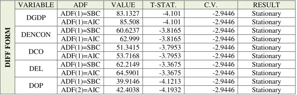
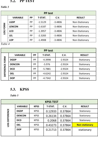
[image:10.595.9.527.375.540.2]determine stationarity. The results of the ADF test, PP tests and KPSS tests are displayed in
table 2,3 and 4 respectively. The test results of ADF and PP below indicate that all the
variables are stationary after first difference except DEL found in the KPSS test was found to
be non-stationary after the first difference. This result gives support to the application of
ARDL bounds method to find out the long-run relationships among the variables. Even
though ARDL has a few drawbacks, it’s still regarded as one of the best time series and is
implemented widely in the world of economics
5.1. ADF Test
Table 2
L
OG
FORM
VARIABLE ADF VALUE T-STAT. C.V. RESULT
LGDP ADF(1)=SBC 84.4865 -1.5294 -3.5348 Non-Stationary
ADF(1)=AIC 87.7083 -1.5294 -3.5348 Non-Stationary
LENCON ADF(1)=SBC 64.4798 -2.2927 -3.5348 Non-Stationary
ADF(1)=AIC 67.7016 -2.2927 -3.5348 Non-Stationary
LCO ADF(1)=SBC 89.2331 -2.4107 -3.5348 Non-Stationary
ADF(1)=AIC 94.6522 -2.4107 -3.5348 Non-Stationary
LEL ADF(1)=SBC 67.949 -2.109 -3.5348 Non-Stationary
ADF(1)=AIC 71.1709 -2.109 -3.5348 Non-Stationary
LOP ADF(1)=SBC 41.2044 -1.8747 -3.5348 Non-Stationary
ADF(1)=AIC 44.4263 -1.8747 -3.5348 Non-Stationary
DIF
F FORM
VARIABLE ADF VALUE T-STAT. C.V. RESULT
DGDP ADF(1)=SBC 83.1327 -4.101 -2.9446 Stationary ADF(1)=AIC 85.508 -4.101 -2.9446 Stationary
DENCON ADF(1)=SBC 60.6237 -3.8165 -2.9446 Stationary ADF(1)=AIC 62.999 -3.8165 -2.9446 Stationary
DCO ADF(1)=SBC 51.3415 -3.7953 -2.9446 Stationary ADF(1)=AIC 53.7168 -3.7953 -2.9446 Stationary
DEL ADF(1)=SBC 62.2149 -3.3675 -2.9446 Stationary ADF(1)=AIC 64.5901 -3.3675 -2.9446 Stationary
[image:10.595.25.526.576.736.2]10
[image:11.595.69.441.77.612.2]5.2.
PP TEST
Table 3
PP test
LOG FORM
VARIABLE PP T-STAT. C.V. RESULT
LGDP PP -1.5129 -3.4806 Non-Stationary
LENCON PP -1.6187 -3.4806 Non-Stationary
LCO PP -1.3957 -3.4806 Non-Stationary
LEL PP -2.3283 -3.4806 Non-Stationary
LOP PP -1.4908 -3.4806 Non-Stationary
Table 4
PP test
D
IF
FE
R
E
N
CE
FOR
M
VARIABLE PP T-STAT. C.V. RESULT
DGDP PP -4.3998 -2.9324 Stationary
DENCON PP -5.976 -2.9324 Stationary
DCO PP -5.7881 -2.9324 Stationary
DEL PP -4.6242 -2.9324 Stationary
DOP PP -4.7342 -2.9324 Stationary
5.3.
KPSS
Table 5
KPSS TEST
LOG DI
FFE
R
E
N
CE
VARIABLE KPSS T-STAT. C.V. RESULT
DGDP KPSS 0.12933 0.37864 Stationary
DENCON KPSS 0.26134 0.37864 Stationary
DCO KPSS 0.2068 0.37864 Stationary
DEL KPSS 0.43273 0.37864 Non stationary
DOP KPSS 0.21713 0.37864 stationary
6.0.
VAR ORDER
The Schwartz-Bayesian Criterion (SBC) and Akaike Information Criterion (AIC) are used to
figure out the optimal number of lags included in the test. Upon analysing, both the AIC and
11 Table 6
Order AIC SBC p-Value C.V.
1 364.665 340.101 [.000] 5%
7.0.
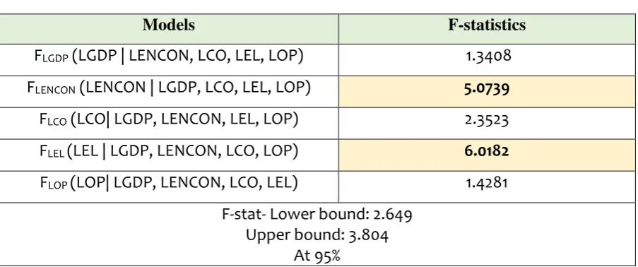
F-TEST Long Run Relation.
Cointegration test indicates the presence of long-run equilibrium relationship, it demonstrates
whether a long run relationship among the variables in this paper are present or not. In each
of the following equations depicted below, the null hypothesis of no cointegration is applied
against the alternative hypothesis of cointegration. The generated F-statistic is compared with
the critical values given by Pesaran et al. (2001). If our F-statistic is higher than the upper
bound level, the null hypothesis is rejected. This entails that the variables are cointegrated. However, if the calculated F-statistic is below the lower bound level, it can be said that the
null hypothesis stands, there is no cointegration. Nonetheless, if the F-statistic falls within the
lower and upper bound level, the results are deemed inconclusive. Our results of the F-test for
[image:12.595.73.525.419.608.2]cointegration are presented in Table 7.
Table 7
Models F-statistics
FLGDP (LGDP | LENCON, LCO, LEL, LOP) 1.3408
FLENCON (LENCON | LGDP, LCO, LEL, LOP) 5.0739
FLCO (LCO| LGDP, LENCON, LEL, LOP) 2.3523
FLEL (LEL | LGDP, LENCON, LCO, LOP) 6.0182
FLOP (LOP| LGDP, LENCON, LCO, LEL) 1.4281
F-stat- Lower bound: 2.649 Upper bound: 3.804
At 95%
The ARDL bound test above in table 7 reveals that not all the 5 estimated models are
cointegrated as only two models have estimated F-statistics well above the upper bounds of
critical value at 95% significance level (2.649 – 3.804). When GDP is taken as a
12
relationship as the calculated F-statistic (1.3408) falls below the lower bound. However, we
did find out that there were long run relationships when LENCON (5.0739), LEL (6.0182)
were set as the dependent variables.
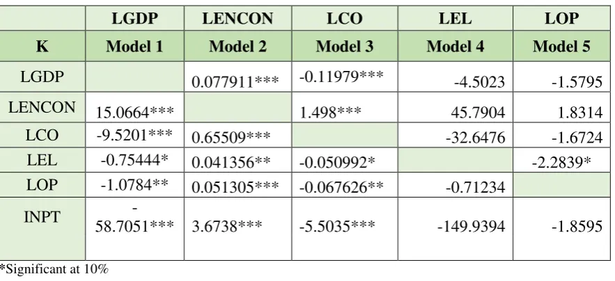
8.0. Results of Estimated Long-Run Coefficients using the ARDL Approach:
[image:13.595.73.515.241.443.2]LONG RUN AIC Table 8
LGDP LENCON LCO LEL LOP
K Model 1 Model 2 Model 3 Model 4 Model 5
LGDP 0.077911*** -0.11979*** -4.5023 -1.5795
LENCON 15.0664*** 1.498*** 45.7904 1.8314 LCO -9.5201*** 0.65509*** -32.6476 -1.6724 LEL -0.75444* 0.041356** -0.050992* -2.2839* LOP -1.0784** 0.051305*** -0.067626** -0.71234
INPT
-58.7051*** 3.6738*** -5.5035*** -149.9394 -1.8595
*Significant at 10% **Significant at 5% ***Significant at 1%
The above table shows that there is a long run relationship between energy consumption and
GDP. They are both positive and highly significant at 1%. That means a 1% increase in
energy consumption would increase GDP by 15.06%. This supports several studies such as
the Jevon’s paradox and Khan and Qayyum (2006) that found a positive relationship between energy consumption and GDP. Therefore, energy consumption plays an important part in
generating economic growth. The same can be said about GDP, a 1% increase in GDP
increases energy consumption only by 0.07 %. In regards to the relationship between trade
and carbon emission, it seems that both have a negative and significant long run relationship.
a 1% increase in trade, reduces carbon emission by about 1.07%, this means open trade
environments have been quite conducive to mitigating carbon emission. However, the same
cannot be said about energy consumption, energy consumption shares a positive and
significant relationship with carbon emission. A 1% rise in energy consumption would lead to
13
(2013), who found that energy consumption plays a vital role in the degradation of the
environment whilst trade openness mitigates the deterioration of the environment. On the
relationship between energy consumption and carbon emissions, the figure shows that an
increase in energy consumption leads to an increase in CO2 emissions. Specifically, a 1%
increase in energy consumption leads to 0.655% increase in carbon emission(pollution). This result supports the view that energy consumption is the main factor of carbon emissions. This
implies that reducing energy consumption, especially the consumption of fossil fuels, is a
feasible option that can aid to reduce carbon dioxide emissions. This is particularly important
because about 70% of South Africa's total primary energy supply is derived from coal, and
coal-fired power stations provide more than 93% of electricity production (World
Bank,2008). Interestingly, we find that trade openness and GDP share a negative and
significant relationship. Specifically, a 1% increase in trade would lead to a decline in GDP
by 1.07%. Even though this goes against previous studies, Feenstra (1990), Matsuyama
(1992) demonstrated that countries lacking technological development can be guided by trade
to concentrate in traditional goods and this would lead to a contraction in economic growth.
9.0.Error Correction Model of ARDL
In the following table, the ECM’s representation for the ARDL model is selected with AIC
[image:14.595.11.594.467.559.2]Criterion.
Table 9: Error Correction Model of ARDL
ecm1(-1) Coefficient Standard Error T-Ratio [Prob.] Significance C.V. Result
DLGDP -0.32243 0.16805 -1.9186[.079] significant 10% endogenous
DLENCON -4.0432 0.86847 -4.6555[.001] significant 1% endogenous
DLCO -3.9159 0.78984 -4.9578[.000] significant 1% endogenous
DLEL -.22009 0.26777 -.82193[.427] not significant 5% exogenous
DLOP 0.91841 0.66241 1.3865[.193] not significant 5% exogenous
As discussed before, cointegration reveals that there is a long run relationship between the
variables but it cannot distinguish the endogeneity or exogeneity of the variables. This is
handled by the error correction model. Since there could be a short-run deviation from the
long-run equilibrium. Cointegration does not disclose the process of short-run adjustment to
bring about the long-run equilibrium. To get a grasp of the adjustment process we need to
proceed to the error-correction model (Table 9). the results reveal that all variables are
endogenous except for trade openness which is exogenous at 5% significance and electricity
consumption at 5% significance. The exogenous variables would receive market
14
us how long it will take to get back to long term equilibrium if that variable is shocked. This
means when we shock trade and electricity consumption which are shown to be the leader
variables, the followers like GDP, carbon emission and energy consumption will be affected.
Thus, it is imperative for policymakers to take better care of the said variables that will have a
profound effect on the country’s economy as a whole. Although the ECM model tends to show the absolute endogeneity and exogeniety of a variable, they do not give us the relative
degree of endogeneity or exogeneity. For that, we need to proceed to the variance
decomposition technique (VDC) to recognize the relativity of these variables.
10.0.
Variance Decomposition (VDC)
Variance decomposition finds out to what extent shocks to specified variables are explained
by other variables in the system. Variance decomposition measures the amount of forecast
error variance in a variable that is explained by innovations or impulse in it and by the other
variables in the system. For instance, it discloses to what proportions of the changes in a
particular variable can be associated to changes in the other lagged explanatory variables.
Moreover, if a variable explains most of its own shock i.e exogenous, then it does not permit
variances of other variables to assist to its explanation and is therefore said to relatively
exogenous. There are two types of VDC that is orthogonalized and generalized. The
difference between these two is that in orthogonalized forecast error variance decomposition,
the amount of percentage of the forecast error variance of a variable which is counted for by
the innovation of another variable in the VAR will sum to one across all the variables. On the
other hand, generalized forecast error VDC permits one to make robust correlation of the
strength, size and persistence of shocks from one equation to another (Payne, 2002) and for
that reason we employ generalized VDC as opposed to orthogonalized VDC. According to
table 10, it can be seen that in the 5-year horizon, trade openness is the most exogenous while
energy consumption is shown to be the most endogenous. These standing remained well pass
15 years. However, in the 20-year horizon, trade still remained the most exogenous.
However, it seems GDP and energy consumption became more exogenous and electricity
consumption became the most endogenous.This indicates that trade has an impact on not
15
Horizon LGDP LENCON LCO LEL LOP TOTAL RANK
LGDP 5 66% 12% 5% 13% 3% 100% 3
LENCON 5 6% 42% 47% 4% 2% 100% 5
LCO 5 4% 42% 49% 4% 1% 100% 4 LEL 5 14% 6% 5% 74% 1% 100% 2
LOP 5 2% 0% 3% 1% 94% 100% 1
Horizon LGDP LENCON LCO LEL LOP Total Ranking
LGDP 10 66% 12% 5% 13% 3% 100% 3
LENCON 10 6% 41% 47% 4% 2% 100% 5 LCO 10 4% 42% 49% 4% 1% 100% 4
LEL 10 14% 6% 5% 74% 1% 100% 2
LOP 10 2% 0% 3% 1% 94% 100% 1
Horizon LGDP LENCON LCO LEL LOP Total Ranking
LGDP 15 66% 12% 5% 13% 3% 100% 3
LENCON 15 6% 41% 47% 4% 2% 100% 5
LCO 15 4% 42% 49% 4% 1% 100% 4
LEL 15 14% 6% 5% 74% 1% 100% 2
LOP 15 2% 0% 3% 1% 94% 100% 1
11.0.
Impulse response Function
From the below graph regarding the generalized impulse response function, the generalized
impulse responses therefore, measure a response from an innovation to a variable. It gives us
the same information as VDC but in graphical form. Judging by the graph, it is quite evident
that all the variables seem to take about 2 years in order to normalise after a ‘shock’. It is
Horizon LGDP LENCON LCO LEL LOP Total Ranking
LGDP 20 66% 12% 5% 13% 3% 1 2
LENCON 20 6% 41% 47% 4% 2% 1 4 LCO 20 4% 42% 49% 4% 1% 1 3
LEL 20 4% 42% 49% 4% 1% 1 5
16
interesting to note that the shock of trade and electricity greatly affects the other variables. In
other words, when there is a shock, the endogenous variables are more affected while the
exogenous variables are less effected. Therefore, the trade openness of a country will depends
on the exchange rate of a country. The policymakers will make decision on GDP based on trade
openness because changes in trade openness will give impact on GDP, as trade is a leader variable.
Generalized Impulse Response(s) to one
S.E. shock in the equation for LOP
LGDP
LENCON
LCO
LEL
LOP
Horizon
-0.02 0.00 0.02 0.04 0.06 0.08 0.10
17
Generalized Impulse Response(s) to one
S.E. shock in the equation for LGDP
LGDP
LENCON
LCO
LEL
LOP
Horizon
0.010 0.015 0.020 0.025
18
Generalized Impulse Response(s) to one
S.E. shock in the equation for LEL
LGDP
LENCON
LCO
LEL
LOP
Horizon
-0.01 0.00 0.01 0.02 0.03 0.04 0.05
0 2 4 6 8 10 12 14 16 18 2020
Generalized Impulse Response(s) to one
S.E. shock in the equation for LCO
LGDP
LENCON
LCO
LEL
LOP
Horizon
0.00 0.01 0.02 0.03 0.04 0.05 0.06
19
12.0.
Persistence Profile (PP)
The graph below presents the persistence profile from a system wide shock it shows that if
the whole cointegrating relationship is shocked, it will take approximately 2 years for the
equilibrium to be re-established.
Generalized Impulse Response(s) to one
S.E. shock in the equation for LENCON
LGDP
LENCON
LCO
LEL
LOP
Horizon
-0.01 0.00 0.01 0.02 0.03 0.04 0.05 0.06
0 2 4 6 8 10 12 14 16 18 2020
Persistence Profile of the effect
of a system-wide shock to CV'(s)
CV1
Horizon
0.0 0.2 0.4 0.6 0.8 1.0
20 13.0. Conclusion and policy implication.
This paper investigated the relationship between economic growth and energy consumption as well as electricity use, trade and carbon dioxide emission using annual time series data covering the period of 1971 – 2013 of South Africa. The results suggest that there is co-integration among the variables. However, it is interesting to note that trade openness and electricity consumption became the leader variable, leaving the rest of the variables endogenous. Even though most studies suggest trade promotes economic growth, we can argue that poor economic growth in South Africa between the years 1993-2002 through to 2013 may have been afflicted by relatively trade polices compared to those in the
BRICS(brazil, Russia, India, China, South Africa) and these policies played somewhat of a role in negatively affecting economic growth. To add, Moon (1998) argues that the
unbalanced specialisation of a certain product, which arises from an outward-oriented
paradigm, may shock economic growth. Thus, it is imperative for policymakers to take better care of these two strong variables as they will have a profound impact on the country’s economy as a whole. In other word, the policymakers will make decision on GDP based on trade openness because changes in trade openness will impact on GDP, as trade is a leader variable. The challenge for the South African authorities is to carry on improving and
maintaining the trade openness policy in order to sustain economic growth and development.
Electricity consumption is the second exogenous variable in our study, thus, the government and policy makers should also advocate and promote restructuring of the electricity supply industry. This may lead to more supply of electricity as more players will be allowed entry into this industry. Therefore, the policymakers should select electricity policies which will support economic growth and reduce environmental pollution in South Africa.
21 REFERENCES
Abid, Μ., Sebri, Μ. (2012), Energy Consumption-Economic Growth Nexus: Does the Level of Aggregation Matter?, International Journal of Energy Economics and Policy 2(2), 55-62
Adebola, S.S., Shahbaz, M. (2013), Trivariate causality between economic growth, urbanisation and electricity consumption in Angola Cointegration and causality analysis. Energy Policy, 60, 876-884
Ahamad, W., Zaman, K., Rastam, R., Taj, S., Waseem, M., Shabir, M. (2013), Economic growth and energy consumption nexus in Pakistan. South Asian Journal of Global Business Research, 2(2), 251-275
Akpan, U.F., Chuku, C.A. (2011), “Economic Growth and Environmental Degradation in Nigeria: Beyond the Environmental Kuznets Curve”, Department of Economics,
University of Uyo, Nigeria.
Antweiler, W., Copeland, R. B., Taylor, M.S., 2001. Is free trade good for the emissions: 1950-2050? The Review of Economics and Statistics 80, 15-27
Arman, Seyed Aziz and Barzegar, Soheila. (2012).the effect of trade liberalization on energy consumption in developing countries. The first national seminar of environmental
conservation and planning.
Ben Aissa, M.S., Ben Jebli, M., Ben Youssef, S. (2014). Output, renewable energy consumption and trade in Africa. Energy Policy, 66, 11-18.
Esso, L.J., 2010. Threshold cointegration and causality relationship between energy use and growth in seven African countries. Energy Economics 32, 1383-1391..
Fallahi, F. (2011), “Causal relationship between energy consumption (EC) and GDP: a Markov-switching (MS) causality”, Energy, Vol. 36, pp. 4165-4170
Feenstra, R. C. (1996). Trade and uneven growth. Journal of Development Economics, 49(1), 229-256
Ghosh, S. (2002), Electricity consumption and economic growth in India. Energy Policy, 30, 125-129
Gross, C. 2012. Explaining the (Non-) Causality between Energy and Economic growth in the U.S.—A Multivariate Sectoral Analysis. Energy Economics 34(2), 489-499.
Gylfason, T., 2000. Resources, agriculture, and economic growth in economies in transition. CESifo Working Paper, Series No. 313, Center for Economic Studies & Ifo Institute for Economic Research.
Halicioglu, F., 2009. An econometric study of CO2 emissions, energy consumption, income and foreign trade in Turkey. Energy Policy 37, 1156–1164
Halicioglu, F. (2011) “A Dynamic Econometric Study of Income, Energy and Exports in Turkey”, Energy, Vol.36, 3348-3354.
22
Khan, M. A., Khan, M. Z., Zaman, K., & Arif, M. (2014). Global estimates of energy- growth nexus: Application of seemingly unrelated regressions. Renewable and Sustainable Energy Reviews, 29, 63-71.
Kohler, M., 2013. CO2 emissions, energy consumption, income and foreign trade: A South African perspective. Energy Policy 63, 1042–1050.
Jensen, M. (2004) Income volatility in small and developing economies: export concentration matters. WTO. https://www.wto.org/english/res_e/booksp_e/discussion_papers3_e.pd
Masuduzzaman, M. (2013), Electricity Consumption and Economic Growth in Bangladesh: Co-integration and Causality Analysis. Research Study Series No.-FDRS 02/2013
Matsuyama, K. (1992). Agricultural productivity, comparative advantage, and economic growth. Journal of Economic Theory, 58(2), 317- 334.
Mozumder, P., Marathe, A. (2007), Causality relationship between electricity consumption and GDP in Bangladesh. Energy Policy, 35, 395-402.
Odhiambo, N.M. (2009), Electricity consumption and economic growth in South Africa: A trivariate causality test. Energy Economics, 31, 635-640.
Pesaran, M.H., Shin, Y. and Smith, R.J. (2001). “Bounds testing approaches to the
analysis of level relationship”, Journal of Applied Econometrics, Vol. 16: 289–326.
Saidi, K., Hammami, S. (2015), The impact of CO2 emissions and economic growth on energy consumption in 58 countries. Energy Reports, 1, 62-70.