Optimizing Spectral Learning for Parsing

Optimizing Spectral Learning for Parsing

Shashi Narayan and Shay B. Cohen

School of Informatics University of Edinburgh Edinburgh, EH8 9LE, UK

{snaraya2,scohen}@inf.ed.ac.uk

Abstract

We describe a search algorithm for opti-mizing the number of latent states when estimating latent-variable PCFGs with spectral methods. Our results show that contrary to the common belief that the number of latent states for each nontermi-nal in an L-PCFG can be decided in isola-tion with spectral methods, parsing results significantly improve if the number of la-tent states for each nonterminal is globally optimized, while taking into account in-teractions between the different nontermi-nals. In addition, we contribute an empiri-cal analysis of spectral algorithms on eight morphologically rich languages: Basque, French, German, Hebrew, Hungarian, Ko-rean, Polish and Swedish. Our results show that our estimation consistently per-forms better or close to coarse-to-fine expectation-maximization techniques for these languages.

1 Introduction

Latent-variable probabilistic context-free gram-mars (L-PCFGs) have been used in the natural lan-guage processing community (NLP) for syntactic parsing for over a decade. They were introduced in the NLP community by Matsuzaki et al. (2005) and Prescher (2005), with Matsuzaki et al. us-ing the expectation-maximization (EM) algorithm to estimate them. Their performance on syntac-tic parsing of English at that stage lagged behind state-of-the-art parsers.

Petrov et al. (2006) showed that one of the reasons that the EM algorithm does not estimate state-of-the-art parsing models for English is that the EM algorithm does not control well for the model size used in the parser – the number of

la-tent states associated with the various nontermi-nals in the grammar. As such, they introduced a coarse-to-fine technique to estimate the grammar. It splits and merges nonterminals (with latent state information) with the aim to optimize the likeli-hood of the training data. Together with other types of fine tuning of the parsing model, this led to state-of-the-art results for English parsing.

In more recent work, Cohen et al. (2012) de-scribed a different family of estimation algorithms for L-PCFGs. This so-called “spectral” family of learning algorithms is compelling because it offers a rigorous theoretical analysis of statistical conver-gence, and sidesteps local maxima issues that arise with the EM algorithm.

While spectral algorithms for L-PCFGs are compelling from a theoretical perspective, they have been lagging behind in their empirical results on the problem of parsing. In this paper we show that one of the main reasons for that is that spectral algorithms require a more careful tuning proce-dure for the number of latent states than that which has been advocated for until now. In a sense, the relationship between our work and the work of Cohen et al. (2013) is analogous to the relation-ship between the work by Petrov et al. (2006) and the work by Matsuzaki et al. (2005): we suggest a technique for optimizing the number of latent states for spectral algorithms, and test it on eight languages.

Our results show that when the number of la-tent states is optimized using our technique, the parsing models the spectral algorithms yield per-form significantly better than the vanilla-estimated models, and for most of the languages – better than the Berkeley parser of Petrov et al. (2006).

As such, the contributions of this parser are two-fold:

• We describe a search algorithm for

ing the number of latent states for spectral learning.

• We describe an analysis of spectral algo-rithms on eight languages (until now the re-sults of L-PCFG estimation with spectral al-gorithms for parsing were known only for English). Our parsing algorithm is rather language-generic, and does not require sig-nificant linguistically-oriented adjustments.

In addition, we dispel the common wisdom that more data is needed with spectral algorithms. Our models yield high performance on treebanks of varying sizes from 5,000 sentences (Hebrew and Swedish) to 40,472 sentences (German).

The rest of the paper is organized as follows. In §2 we describe notation and background. §3 further investigates the need for an optimization of the number of latent states in spectral learn-ing and describes our optimization algorithm, a search algorithm akin to beam search. In§4 we de-scribe our experiments with natural language pars-ing for Basque, French, German, Hebrew, Hungar-ian, Korean, Polish and Swedish. We conclude in

§5.

2 Background and Notation

We denote by [n] the set of integers {1, . . . , n}. An L-PCFG is a 5-tuple(N,I,P, f, n)where:

• N is the set of nonterminal symbols in the grammar. I ⊂ N is a finite set of intermi-nals. P ⊂ N is a finite set ofpreterminals. We assume thatN =I ∪ P, andI ∩ P =∅. Hence we have partitioned the set of nonter-minals into two subsets.

• f:N →Nis a function that maps each non-terminal a to the number of latent states it uses. The set[ma]includes the possible hid-den states for nonterminala.

• [n]is the set of possible words.

• For alla ∈ I, b ∈ N,c ∈ N, h1 ∈ [ma],

h2 ∈ [mb], h3 ∈ [mc], we have a binary context-free rulea(h1)→b(h2) c(h3). • For alla∈ P,h ∈[ma],x ∈[n], we have a

lexical context-free rulea(h)→x.

The estimation of an L-PCFG requires an as-signment of probabilities (or weights) to each of

the rules a(h1) → b(h2) c(h3)and a(h) → x,

and also an assignment of starting probabilities for eacha(h), wherea ∈ I andh ∈ [ma]. Estima-tion is usually assumed to be done from a set of parse trees (a treebank), where the latent states are not included in the data – only the “skeletal” trees which consist of nonterminals inN.

L-PCFGs, in their symbolic form, are related to regular tree grammars, an old grammar formal-ism, but they were introduced as statistical mod-els for parsing with latent heads more recently by Matsuzaki et al. (2005) and Prescher (2005). Earlier work about L-PCFGs by Matsuzaki et al. (2005) used the expectation-maximization (EM) algorithm to estimate the grammar probabilities. Indeed, given that the latent states are not ob-served, EM is a good fit for L-PCFG estimation, since it aims to do learning from incomplete data. This work has been further extended by Petrov et al. (2006) to use EM in a coarse-to-fine fashion: merging and splitting nonterminals using the la-tent states to optimize the number of lala-tent states for each nonterminal.

Cohen et al. (2012) presented a so-called spec-tral algorithm to estimate L-PCFGs. This algo-rithm uses linear-algebraic procedures such as sin-gular value decomposition (SVD) during learning. The spectral algorithm of Cohen et al. builds on an estimation algorithm for HMMs by Hsu et al. (2009).1 _{Cohen et al. (2013) experimented with}

this spectral algorithm for parsing English. A dif-ferent variant of a spectral learning algorithm for L-PCFGs was developed by Cohen and Collins (2014). It breaks the problem of L-PCFG estima-tion into multiple convex optimizaestima-tion problems which are solved using EM.

The family of L-PCFG spectral learning algo-rithms was further extended by Narayan and Co-hen (2015). They presented a simplified version of the algorithm of Cohen et al. (2012) that es-timates sparse grammars and assigns probabili-ties (instead of weights) to the rules in the gram-mar, and as such does not suffer from the prob-lem of negative probabilities that arise with the original spectral algorithm (see discussion in Co-hen et al., 2013). In this paper, we use the algo-rithms by Narayan and Cohen (2015) and Cohen

1_{A related algorithm for weighted tree automata (WTA)}

VP V chased

NP D the

N cat

S NP D the

N mouse

VP

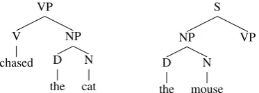
Figure 1: The inside tree (left) and outside tree (right) for the nonterminal VP in the parse tree (S (NP (D the) (N mouse)) (VP (V chased) (NP (D the) (N cat)))) for the sentence“the mouse chased the cat.”

et al. (2012), and we compare them against state-of-the-art L-PCFG parsers such as the Berkeley parser (Petrov et al., 2006). We also compare our algorithms to other state-of-the-art parsers where elaborate linguistically-motivated feature specifi-cations (Hall et al., 2014), annotations (Crabb´e, 2015) and formalism conversions (Fern´andez-Gonz´alez and Martins, 2015) are used.

3 Optimizing Spectral Estimation

In this section, we describe our optimization algo-rithm and its motivation.

3.1 Spectral Learning of L-PCFGs and Model Size

The family of spectral algorithms for latent-variable PCFGs rely on feature functions that are defined forinsideandoutsidetrees. Given a tree, the inside tree for a node contains the entire sub-tree below that node; the outside sub-tree contains ev-erything in the tree excluding the inside tree. Fig-ure 1 shows an example of inside and outside trees for the nonterminalVPin the parse tree of the sen-tence“the mouse chased the cat”.

With L-PCFGs, the model dictates that an in-side tree and an outin-side tree that are connected at a node are statistically conditionally independent of each other given the node label and the latent state that is associated with it. As such, one can identify the distribution over the latent states for a given nonterminalaby using the cross-covariance matrix of the inside and the outside trees,Ωa_{. For} more information on the definition of this cross-covariance matrix, see Cohen et al. (2012) and Narayan and Cohen (2015).

The L-PCFG spectral algorithms use singular value decomposition (SVD) onΩa _{to reduce the} dimensionality of the feature functions. IfΩa _is computed from the true L-PCFG distribution then

the rank of Ωa _{(the number of non-zero singular} values) gives the number of latent states according to the model.

In the case of estimating Ωa _{from data} gener-ated from an L-PCFG, the number of latent states for each nonterminal can be exposed by capping it when the singular values ofΩa_{are smaller than} some threshold value. This means that spectral al-gorithms give a natural way for the selection of the number of latent states for each nonterminalain the grammar.

However, when the data from which we esti-mate an PCFG model are not drawn from an L-PCFG (the model is “incorrect”), the number of non-zero singular values (or the number of singu-lar values which are singu-large) is no longer sufficient to determine the number of latent states for each nonterminal. This is where our algorithm comes into play: it optimizes the number of latent search for each nonterminal by applying a search algo-rithm akin to beam search.

3.2 Optimizing the Number of Latent States

As mentioned in the previous section, the number of non-zero singular values ofΩa_{gives a criterion} to determine the number of latent statesmafor a given nonterminala. In practice, we capmanot to include small singular values which are close to 0, because of estimation errors ofΩa_.

up-Inputs: An input treebank divided into training and devel-opment set. A basic spectral estimation algorithmSwith its default setting. An integerkdenoting the size of the beam. An integermdenoting the upper bound on the number of latent states.

Algorithm:

(Step 0: Initialization)

• SetQ, a queue of sizek, to be empty.

• Estimate an L-PCFGGS: (N,I,P, fS, n)usingS.

• Initializef=fS, a function that maps each

nontermi-nala∈ N to the number of latent states.

• LetLbe a list of nonterminals(a1, . . . , aM)such that

ai ∈ N for which to optimize the number of latent

states.

• Letsbe theF1score for the above L-PCFGGSon the

development set.

• Put inQthe element(s,1, f,coarse).

• The queue is ordered bys, the first element of tuples, in the queue.

(Step 1: Search, repeat until termination happens)

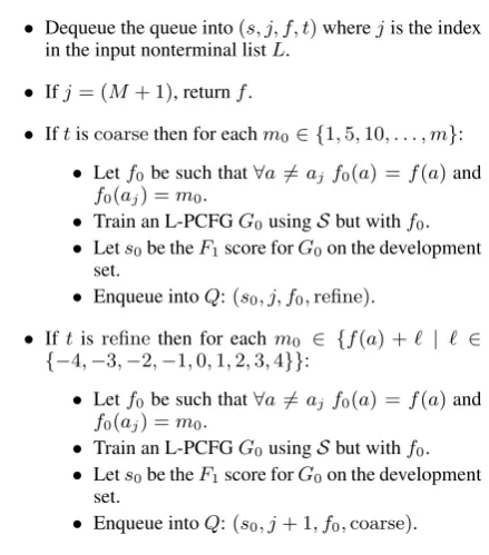
• Dequeue the queue into(s, j, f, t)wherejis the index in the input nonterminal listL.

• Ifj= (M+ 1), returnf.

• Iftiscoarsethen for eachm0∈ {1,5,10, . . . , m}:

• Letf0be such that∀a 6=ajf0(a) =f(a)and

f0(aj) =m0.

• Train an L-PCFGG0usingSbut withf0.

• Lets0be theF1score forG0on the development set.

• Enqueue intoQ:(s0, j, f0,refine).

• Iftisrefinethen for eachm0 ∈ {f(a) +` | ` ∈

{−4,−3,−2,−1,0,1,2,3,4}}:

• Letf0be such that∀a6=ajf0(a) =f(a)and

f0(aj) =m0.

• Train an L-PCFGG0usingSbut withf0.

• Lets0be theF1score forG0on the development set.

• Enqueue intoQ:(s0, j+ 1, f0,coarse).

Figure 2: A search algorithm for finding the opti-mal number of latent states.

per bound to keep the grammar size small. Petrov et al. (2006) improves over the estima-tion described in Matsuzaki et al. (2005) by taking into account the interactions between the nonter-minals and their latent state numbers in the train-ing data. They use the EM algorithm to split and merge nonterminals using the latent states, and

op-timize the number of latent states for each nonter-minal such that it maximizes the likelihood of a training treebank. Their refined grammar success-fully splits nonterminals to various degrees to cap-ture their complexity. We take the analogous step with spectral methods. We propose an algorithm where we first compute Ωa _{on the training data} and then we optimize the number of latent states for each nonterminal by optimizing the PARSE-VAL metric (Black et al., 1991) on a development set.

Our optimization algorithm appears in Figure 2. The input to the algorithm is training and develop-ment data in the form of parse trees, a basic spec-tral estimation algorithm S in its default setting, an upper boundm on the number of latent states that can be used for the different nonterminals and a beam sizekwhich gives a maximal queue size for the beam. The algorithm aims to learn a func-tionfthat maps each nonterminalato the number of latent states. It initializesf by estimating a de-fault grammarGS : (N,I,P, fS, n)usingS and

settingf = fS. It then iterates overa ∈ N,

im-provingf such that it optimizes the PARSEVAL metric on the development set.

The state of the algorithm includes a queue that consists of tuples of the form (s, j, f, t) where f

is an assignment of latent state numbers to each nonterminal in the grammar, j is the index of a nonterminal to be explored in the input nontermi-nal listL,sis theF1score on the development set for a grammar that is estimated withf andtis a tag that can either becoarseorrefine.

The algorithm orders these tuples by s in the queue, and iteratively dequeues elements from the queue. Then, depending on the labelt, it either makes a refined search for the number of latent states for aj, or a more coarse search. As such, the algorithm can be seen as a variant of a beam search algorithm.

The search algorithm can be used with any training algorithm for L-PCFGs, including the al-gorithms of Cohen et al. (2013) and Narayan and Cohen (2015). These methods, in their default set-ting, use a function fS which maps each

lang. Basque French German-N German-T Hebrew Hungarian Korean Polish Swedish

train

sent. 7,577 14,759 18,602 40,472 5,000 8,146 23,010 6,578 5,000

tokens 96,565 443,113 328,531 719,532 128,065 170,221 301,800 66,814 76,332

lex. size 25,136 27,470 48,509 77,219 15,971 40,775 85,671 21,793 14,097

#nts 112 222 208 762 375 112 352 198 148

de

v sent. 948 1,235 1,000 5,000 500 1,051 2,066 821 494

tokens 13,893 38,820 17,542 76,704 11,305 30,010 25,729 8,391 9,339

test sent.tokens 11,477946 75,2162,541 17,5851,000 92,0045,000 17,002716 19,9131,009 28,7832,287 8,336822 10,675666

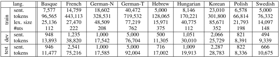
Table 1:Statistics about the different datasets used in our experiments for the training (“train”), development (“dev”) and test (“test”) sets. “sent.” denotes the number of sentences in the dataset, “tokens” denotes the total number of words in the dataset, “lex. size” denotes the vocabulary size in the training set and “#nts” denotes the number of nonterminals in the training set after binarization.

SVD on the cross-covariance matrixΩaof the in-side and the outin-side trees, for each nonterminala. Cohen et al. (2013) estimate the parameters of the L-PCFG up to a linear transformation usingf(a) non-zero singular values ofΩa, whereas Narayan and Cohen (2015) use the feature representations induced from the SVD step to cluster instances of nonterminalain the training data intof(a) clus-ters; these clusters are then treated as latent states that are “observed.” Finally, Narayan and Cohen follow up with a simple frequency count maxi-mum likelihood estimate to estimate the parame-ters in the L-PCFG with these latent states.

An important point to make is that the learning algorithms of Narayan and Cohen (2015) and Co-hen et al. (2013) are relatively fast,2_{in comparison}

to the EM algorithm. They require only one iter-ation over the data. In addition, the SVD step of

S for these learning algorithms is computed just once for a largem. The SVD of a lower rank can then be easily computed from that SVD.

4 Experiments

In this section, we describe our setup for parsing experiments on a range of languages.

4.1 Experimental Setup

Datasets We experiment with nine treebanks consisting of eight different morphologically rich languages: Basque, French, German, Hebrew, Hungarian, Korean, Polish and Swedish. Table 1 shows the statistics of 9 different treebanks with their splits into training, development and test sets. Eight out of the nine datasets (Basque, French, German-T, Hebrew, Hungarian, Korean, Polish

2_{It has been documented in several papers that the}

fam-ily of spectral estimation algorithms is faster than algorithms such as EM, not just for L-PCFGs. See, for example, Parikh et al. (2012).

and Swedish) are taken from the workshop on Statistical Parsing of Morphologically Rich Lan-guages (SPMRL; Seddah et al., 2013). The Ger-man corpus in the SPMRL workshop is taken from the TiGer corpus (German-T, Brants et al., 2004). We also experiment with another German cor-pus, the NEGRA corpus (German-N, Skut et al., 1997), in a standard evaluation split.3 _{Words in}

the SPMRL datasets are annotated with their mor-phological signatures, whereas the NEGRA cor-pus does not contain any morphological informa-tion.

Data preprocessing and treatment of rare words We convert all trees in the treebanks to a binary form, train and run the parser in that form, and then transform back the trees when doing eval-uation using the PARSEVAL metric. In addition, we collapse unary rules into unary chains, so that our trees are fully binarized. The column “#nts” in Table 1 shows the number of nonterminals af-ter binarization in the various treebanks. Before binarization, we also drop all functional informa-tion from the nonterminals. We use fine tags for all languages except Korean. This is in line with Bj¨orkelund et al. (2013).4 _{For Korean, there are}

2,825 binarized nonterminals making it impracti-cal to use our optimization algorithm, so we use the coarse tags.

Bj¨orkelund et al. (2013) have shown that the morphological signatures for rare words are useful to improve the performance of the Berkeley parser.

3_{We use the first 18,602 sentences as a training set, the}

next 1,000 sentences as a development set and the last 1,000 sentences as a test set. This corresponds to an 80%-10%-10% split of the treebank.

4_{In their experiments Bj¨orkelund et al. (2013) found that}

In our preliminary experiments with na¨ıve spectral estimation, we preprocess rare words in the train-ing set in two ways: (i) we replace them with their corresponding POS tags, and (ii) we replace them with their corresponding POS+morphological sig-natures. We follow Bj¨orkelund et al. (2013) and consider a word to be rare if it occurs less than 20 times in the training data. We experimented both with a version of the parser that does not ignore and does ignore letter cases, and discovered that the parser behaves better when case is not ignored.

Spectral algorithms: subroutine choices The latent state optimization algorithm will work with either the clustering estimation algorithm of Narayan and Cohen (2015) or the spectral algo-rithm of Cohen et al. (2013). In our setup, we first run the latent state optimization algorithm with the clustering algorithm. We then run the spectral algorithm once with the optimizedf from the clustering algorithm. We do that because the clustering algorithm is significantly faster to itera-tively parse the development set, because it leads to sparse estimates.

Our optimization algorithm is sensitive to the initialization of the number of latent states as-signed to each nonterminals as it sequentially goes through the list of nonterminals and chooses latent state numbers for each nonterminal, keeping latent state numbers for other nonterminals fixed. In our setup, we start our search algorithm with the best model from the clustering algorithm, controlling for all hyperparameters; we tune f, the function which maps each nonterminal to a fixed number of latent statesm, by running the vanilla version with different values ofmfor different languages. Based on our preliminary experiments, we setm

to 4 for Basque, Hebrew, Polish and Swedish; 8 for German-N; 16 for German-T, Hungarian and Korean; and 24 for French.

We use the same features for the spectral meth-ods as in Narayan and Cohen (2015) for German-N. For the SPMRL datasets we do not use the head features. These require linguistic understanding of the datasets (because they require head rules for propagating leaf nodes in the tree), and we discov-ered that simple heuristics for constructing these rules did not yield an increase in performance.

We use the kmeans function in Matlab to do the clustering for the spectral algorithm of Narayan and Cohen (2015). We experimented with several versions ofk-means, and discovered

that the version that works best in a set of prelimi-nary experiments is hardk-means.5

Decoding and evaluation For efficiency, we use a base PCFG without latent states to prune marginals which receive a value less than0.00005 in the dynamic programming chart. This is just a bare-bones PCFG that is estimated using maximum likelihood estimation (with frequency count). The parser takes part-of-speech tagged sentences as input. We tag the German-N data us-ing the Turbo Tagger (Martins et al., 2010). For the languages in the SPMRL data we use the Mar-Mot tagger of M¨ueller et al. (2013) to jointly pre-dict the POS and morphological tags.6 _{The parser}

itself can assign different part-of-speech tags to words to avoid parse failure. This is also particu-larly important for constituency parsing with mor-phologically rich languages. It helps mitigate the problem of the taggers to assign correct tags when long-distance dependencies are present.

For all results, we report the F1 measure of the PARSEVAL metric (Black et al., 1991). We use the EVALB program7 _{with the}

parame-ter file COLLINS.prm (Collins, 1999) for the German-N data and the SPMRL parameter file, spmrl.prm, for the SPMRL data (Seddah et al., 2013).

In this setup, the latent state optimization algo-rithm terminates in few hours for all datasets ex-cept French and German-T. The German-T data has 762 nonterminals to tune over a large develop-ment set consisting of 5,000 sentences, whereas, the French data has a high average sentence length of 31.43 in the development set.8

Following Narayan and Cohen (2015), we fur-ther improve our results by using multiple spec-tral models where noise is added to the underlying features in the training set before the estimation of each model.9 _{Using the optimizedf, we estimate} 5_{To be more precise, we use the Matlab functionkmeans}

while passing it the parameter‘start’=‘sample’to ran-domly sample the initial centroid positions. In our experi-ments, we found that default initialization of centroids differs in Matlab14 (random) and in Matlab15 (kmeans++). Our es-timation performs better with random initialization.

6_{See Bj¨orkelund et al. (2013) for the performance of the}

MarMot tagger on the SPMRL datasets.

7_{http://nlp.cs.nyu.edu/evalb/}

8_{To speed up tuning on the French data, we drop sentences}

with length>46 from the development set, dropping its size from 12,35 to 1,006.

9_{We only use the algorithm of Narayan and Cohen (2015)}

lang. Basque French German-N German-T Hebrew Hungarian Korean Polish Swedish Bk van_rep 69.2_84.3 79.9_79.7 -_{- 82.7}81.7 87.8_89.6 83.9_{89.1 82.8}71.0 _87.184.1 74.5_75.5

Cl van (pos)van (rep) 69.878.6 73.973.7 75.7- 78.878.3 88.088.1 81.384.7 76.568.7 90.490.3 70.971.4

opt 81.2∗ _{76.7 77.8 81.7 90.1 87.2 79.2 92.0 75.2}

Sp _optvan 78.1_{79.0 78.1}78.0∗ _79.077.6∗ _82.982.0∗ _90.389.2∗ _87.887.7∗ _80.980.6∗ _91.791.7∗ _75.573.4∗

Bk multiple 87.4 82.5 - 85.0 90.5 91.1 84.6 88.4 79.5

Cl multiple 83.4 79.9 82.7 85.1 90.6 89.0 80.8 92.5 78.3

Hall et al. ’14 83.7 79.4 - 83.3 88.1 87.4 81.9 91.1 76.0

Crabb´e ’15 84.0 80.9 - 84.1 90.7 88.3 83.1 92.8 77.9

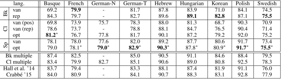
Table 2: Results on the development datasets. “Bk” makes use of the Berkeley parser with its coarse-to-fine mechanism to optimize the number of latent states (Petrov et al., 2006). For Bk, “van” uses the vanilla treatment of rare words using signatures defined by Petrov et al. (2006), whereas “rep.” uses the morphological signatures instead. “Cl” uses the algorithm of Narayan and Cohen (2015) and “Sp” uses the algorithm of Cohen et al. (2013). In Cl, “van (pos)” and “van (rep)” are vanilla estima-tions (i.e., each nonterminal is mapped to fixed number of latent states) replacing rare words by POS or POS+morphological signatures, respectively. The best of these two models is used with our optimization algorithm in “opt”. For Sp, “van” uses the best setting for unknown words as Cl. Best result in each column from the first seven rows is in bold. In addition, our best performing models from rows 3-7 are marked with∗_{. “Bk multiple” shows the best results with the multiple models using}

product-of-grammars procedure (Petrov, 2010) and discriminative reranking (Charniak and Johnson, 2005). “Cl multiple” gives the results with multiple models generated using the noise induction and decoded using the hierarchical decoding (Narayan and Cohen, 2015). Bk results are not available on the development dataset for German-N. For others, we report Bk results from Bj¨orkelund et al. (2013). We also include results from Hall et al. (2014) and Crabb´e (2015).

lang. Basque French German-N German-T Hebrew Hungarian Korean Polish Swedish

Bk 74.7 80.4 80.1 78.3 87.0 85.2 78.6 86.8 80.6

Cl van_{opt 81.4}79.6∗ _75.674.3 76.4_78.0 74.1_76.0 86.3_87.2 86.5_88.4 76.5_78.4 90.5_91.2 76.4_79.4

Sp _optvan 79.9_{80.5 79.1}78.7∗ _79.478.4∗ _78.278.0∗ _89.087.8∗ _89.289.1∗ _80.080.3∗ _91.891.8∗ _80.978.4∗

Bk multiple 87.9 82.9 84.5 81.3 89.5 91.9 84.3 87.8 84.9

Cl multiple 83.4 80.4 82.7 80.4 89.2 89.9 80.3 92.4 82.8

Hall et al. ’14 83.4 79.7 - 78.4 87.2 88.3 80.2 90.7 82.0

F&M ’15 85.9 78.8 - 78.7 89.0 88.2 79.3 91.2 82.8

Crabb´e ’15 84.9 80.8 - 79.3 89.7 90.1 82.7 92.7 83.2

Table 3: Results on the test datasets. “Bk” denotes the best Berkeley parser result reported by the shared task organizers (Seddah et al., 2013). For the German-N data, Bk results are taken from Petrov (2010). “Cl van” shows the performance of the best vanilla models from Table 2 on the test set. “Cl opt” and “Sp opt” give the result of our algorithm on the test set. We also include results from Hall et al. (2014), Crabb´e (2015) and Fern´andez-Gonz´alez and Martins (2015).

80models for each of noise induction mechanisms in Narayan and Cohen: Dropout, Gaussian (ad-ditive) and Gaussian (multiplicative). To decode with multiple noisy models, we train the MaxEnt reranker of Charniak and Johnson (2005).10

Hi-erarchical decoding with “maximal tree coverage” over MaxEnt models, further improves our accu-racy. See Narayan and Cohen (2015) for more de-tails on the estimation of a diverse set of models, and on decoding with them.

estimates than the dense estimates of Cohen et al. (2013).

10_{Implementation: https://github.com/BLLIP/}

bllip-parser. More specifically, we used the programs extract-spfeatures, cvlm-lbfgs and best-indices.extract-spfeaturesuses head fea-tures, we bypass this for the SPMRL datasets by creating a dummyheads.ccfile. cvlm-lbfgswas used with the default hyperparameters from the Makefile.

4.2 Results

Table 2 and Table 3 give the results for the various languages.11 _{Our main focus is on comparing the}

coarse-to-fine Berkeley parser (Petrov et al., 2006) to our method. However, for the sake of com-pleteness, we also present results for other parsers, such as parsers of Hall et al. (2014), Fern´andez-Gonz´alez and Martins (2015) and Crabb´e (2015).

In line with Bj¨orkelund et al. (2013), our pre-liminary experiments with the treatment of rare words suggest that morphological features are useful for all SPMRL languages except French. Specifically, for Basque, Hungarian and Korean, improvements are significantly large.

Our results show that the optimization of the

11_{See more in http://cohort.inf.ed.ac.uk/}

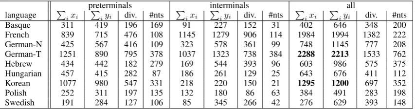
preterminals interminals all

language P

ixi Piyi div. #nts Pixi Piyi div. #nts Pixi Piyi div. #nts

Basque 311 419 196 169 91 227 152 31 402 646 348 200

French 839 715 476 108 1145 1279 906 114 1984 1994 1382 222

German-N 425 567 416 109 323 578 361 99 748 1145 777 208

German-T 1251 890 795 378 1037 1323 738 384 2288 2213 1533 762

Hebrew 434 442 182 279 169 544 393 96 603 986 575 375

Hungarian 457 415 282 87 186 261 129 25 643 676 411 112

Korean 1077 980 547 331 218 220 150 21 1295 1200 697 352

Polish 252 311 197 135 132 180 86 63 384 491 283 198

Swedish 191 284 127 106 85 345 266 42 276 629 393 148

Table 4: A comparison of the number of latent states for the different nonterminals before and after running our latent state number optimization algorithm. The indexiranges over preterminals and interminals, withxidenoting the number of latent

states for nonterminaliwith the vanilla version of the estimation algorithm andyidenoting the number of latent states for

nonterminaliafter running the optimization algorithm. The divergence figure (“div.”) is a calculation ofP

i|xi−yi|.

number of latent states with the clustering and spectral algorithms indeed improves these algo-rithms performance, and these increases general-ize to the test sets as well. This was a point of concern, since the optimization algorithm goes through many points in the hypothesis space of parsing models, and identifies one that behaves op-timally on the development set – and as such it could overfit to the development set. However, this did not happen, and in some cases, the increase in accuracy of the test set after running our optimiza-tion algorithm is actually larger than the one for the development set.

While the vanilla estimation algorithms (with-out latent state optimization) lag behind the Berke-ley parser for many of the languages, once the number of latent states is optimized, our parsing models do better for Basque, Hebrew, Hungar-ian, Korean, Polish and Swedish. For German-T we perform close to the Berkeley parser (78.2 vs. 78.3). It is also interesting to compare the clustering algorithm of Narayan and Cohen (2015) to the spectral algorithm of Cohen et al. (2013). In the vanilla version, the spectral algorithm does better in most cases. However, these differences are narrowed, and in some cases, overcome, when the number of latent states is optimized. Decod-ing with multiple models further improves our ac-curacy. Our “Cl multiple” results lag behind “Bk multiple.” We believe this is the result of the need of head features for the MaxEnt models.12

Our results show that spectral learning is a viable alternative to the use of

expectation-12_{Bj¨orkelund et al. (2013) also use the MaxEnt raranker}

with multiple models of the Berkeley parser, and in their case also the performance after the raranking step is not always significantly better. See footnote 10 on how we create dummy head-features for our MaxEnt models.

maximization coarse-to-fine techniques. As we discuss later, further improvements have been in-troduced to state-of-the-art parsers that are orthog-onal to the use of a specific estimation algorithm. Some of them can be applied to our setup.

4.3 Further Analysis

In addition to the basic set of parsing results, we also wanted to inspect the size of the parsing mod-els when using the optimization algorithm in com-parison to the vanilla models. Table 4 gives this analysis. In this table, we see that in most cases, on average, the optimization algorithm chooses to enlarge the number of latent states. However, for German-T and Korean, for example, the optimiza-tion algorithm actually chooses a smaller model than the original vanilla model.

We further inspected the behavior of the optimization algorithm for the preterminals in German-N, for which the optimal model chose (on average) a larger number of latent states. Table 5 describes this analysis. We see that in most cases, the optimization algorithm chose to decrease the number of latent states for the various pretermi-nals, but in some cases significantly increases the number of latent states.13

Our experiments dispel another “common wis-dom” about spectral learning and training data size. It has been believed that spectral learning do not behave very well when small amounts of data are available (when compared to maximum likelihood estimation algorithms such as EM) – however we see that our results do better than the Berkeley parser for several languages with small

13_{Interestingly, most of the punctuation symbols, such as}

$∗_LRB∗_{,$. and$,, drop their latent state number to a}

preterminal freq. b. a. preterminal freq. b. a. preterminal freq. b. a. preterminal freq. b. a. PWAT 64 2 2 TRUNC 614 8 1 PIS 1,628 8 8 KON 8,633 8 30

XY 135 3 1 VAPP 363 6 4 $*LRB* 13,681 8 6 PPER 4,979 8 100

NP|NN 88 2 1 PDS 988 8 8 ADJD 6,419 8 60 $. 17,699 8 3

VMINF 177 3 5 AVP|ADV 211 4 11 KOUS 2,456 8 1 APPRART 6,217 8 15 PTKA 162 3 1 FM 578 8 3 PIAT 1,061 8 8 ADJA 18,993 8 10 VP|VVINF 409 6 2 VVIMP 76 2 1 NP|PPER 382 6 1 APPR 26,717 8 7 PRELAT 94 2 1 KOUI 339 5 2 VVPP 5,005 8 20 VVFIN 13,444 8 3 AP|ADJD 178 3 1 VAINF 1,024 8 1 PP|PROAV 174 3 1 $, 16,631 8 1

APPO 89 2 2 PRELS 2,120 8 40 VAFIN 8,814 8 1 VVINF 4,382 8 10 PWS 361 6 1 CARD 6,826 8 8 PTKNEG 1,884 8 8 ART 35,003 8 10 KOKOM 800 8 37 NE 17,489 8 6 PTKZU 1,586 8 1 ADV 15,566 8 8 VP|VVPP 844 8 5 PRF 2,158 8 1 VVIZU 479 7 1 PIDAT 1,254 8 20 PWAV 689 8 1 PDAT 1,129 8 1 PPOSAT 2,295 8 6 NN 68,056 8 12 APZR 134 3 2 PROAV 1,479 8 10 PTKVZ 1,864 8 3 VMFIN 3,177 8 1

Table 5:A comparison of the number of latent states for each preterminal for the German-N model, before (“b.”) running the latent state number optimization algorithm and after running it (“a.”). Note that some of the preterminals denote unary rules that were collapsed (the nonterminals in the chain are separated by|). We do not show rare preterminals with b. and a. both being 1.

training datasets, such as Basque, Hebrew, Pol-ish and Hungarian. The source of this common wisdom is that ML estimators tend to be statis-tically “efficient:” they extract more information from the data than spectral learning algorithms do. Indeed, there is no reason to believe that spectral algorithms are statistically efficient. However, it is not clear that indeed for L-PCFGs with the EM algorithm, the ML estimator is statistically effi-cient either. MLE is statistically effieffi-cient under specific assumptions which are not clearly satis-fied with L-PCFG estimation. In addition, when the model is “incorrect,” (i.e. when the data is not sampled from L-PCFG, as we would expect from natural language treebank data), spectral al-gorithms could yield better results because they can mimic a higher order model. This can be understood through HMMs. When estimating an HMM of a low order with data which was gener-ated from a higher order model, EM does quite poorly. However, if the number of latent states (and feature functions) is properly controlled with spectral algorithms, a spectral algorithm would learn a “product” HMM, where the states in the lower order model are the product of states of a higher order.14

State-of-the-art parsers for the SPMRL datasets improve the Berkeley parser in ways which are or-thogonal to the use of the basic estimation algo-rithm and the method for optimizing the number of latent states. They include transformations of the treebanks such as with unary rules (Bj¨orkelund et al., 2013), a more careful handling of unknown words and better use of morphological

informa-14_{For example, a trigram HMM can be reduced to a bigram}

HMM where the states are products of the original trigram HMM.

tion such as decorating preterminals with such in-formation (Bj¨orkelund et al., 2014; Sz´ant´o and Farkas, 2014), with careful feature specifications (Hall et al., 2014) and head-annotations (Crabb´e, 2015), and other techniques. Some of these tech-niques can be applied to our case.

5 Conclusion

We demonstrated that a careful selection of the number of latent states in a latent-variable PCFG with spectral estimation has a significant effect on the parsing accuracy of the L-PCFG. We de-scribed a search procedure to do this kind of optimization, and described parsing results for eight languages (with nine datasets). Our results demonstrate that when comparing the expectation-maximization with coarse-to-fine techniques to our spectral algorithm with latent state optimiza-tion, spectral learning performs better on six of the datasets. Our results are comparable to other state-of-the-art results for these languages. Using a di-verse set of models to parse these datasets further improves the results.

Acknowledgments

References

Rapha¨el Bailly, Amaury Habrard, and Franc¸ois Denis. 2010. A spectral approach for probabilistic gram-matical inference on trees. InProceedings of Inter-national Conference on Algorithmic Learning The-ory.

Anders Bj¨orkelund, ¨Ozlem C¸etino˘glu, Rich´ard Farkas, Thomas M¨ueller, and Wolfgang Seeker. 2013. (Re)ranking meets morphosyntax: State-of-the-art results from the SPMRL 2013 shared task. In Pro-ceedings of the Fourth Workshop on Statistical Pars-ing of Morphologically-Rich Languages.

Anders Bj¨orkelund, ¨Ozlem C¸etino˘glu, Agnieszka Fale´nska, Rich´ard Farkas, Thomas M¨uller, Wolf-gang Seeker, and Zsolt Sz´ant´o. 2014. Introducing the IMS-Wrocław-Szeged-CIS entry at the SPMRL 2014 shared task: Reranking and morphosyntax meet unlabeled data. In Proceedings of the First Joint Workshop on Statistical Parsing of Morpho-logically Rich Languages and Syntactic Analysis of Non-Canonical Languages.

Ezra W. Black, Steven Abney, Daniel P. Flickinger, Claudia Gdaniec, Ralph Grishman, Philip Harri-son, Donald Hindle, Robert J. P. Ingria, Freder-ick Jelinek, Judith L. Klavans, Mark Y. Liberman, Mitchell P. Marcus, Salim Roukos, Beatrice San-torini, and Tomek Strzalkowski. 1991. A procedure for quantitatively comparing the syntactic coverage of English grammars. In Proceedings of DARPA Workshop on Speech and Natural Language. Sabine Brants, Stefanie Dipper, Peter Eisenberg,

Sil-via Hansen-Schirra, Esther K¨onig, Wolfgang Lezius, Christian Rohrer, George Smith, and Hans Uszko-reit. 2004. TIGER: Linguistic interpretation of a German corpus. Research on Language and Com-putation, 2(4):597–620.

Eugene Charniak and Mark Johnson. 2005. Coarse-to-fine n-best parsing and maxent discriminative reranking. InProceedings of ACL.

Shay B. Cohen and Michael Collins. 2014. A prov-ably correct learning algorithm for latent-variable PCFGs. InProceedings of ACL.

Shay B. Cohen, Karl Stratos, Michael Collins, Dean F. Foster, and Lyle Ungar. 2012. Spectral learning of latent-variable PCFGs. InProceedings of ACL. Shay B. Cohen, Karl Stratos, Michael Collins, Dean P.

Foster, and Lyle Ungar. 2013. Experiments with spectral learning of latent-variable PCFGs. In Pro-ceedings of NAACL.

Michael Collins. 1999. Head-Driven Statistical Mod-els for Natural Language Parsing. Ph.D. thesis, University of Pennsylvania.

Benoit Crabb´e. 2015. Multilingual discriminative lex-icalized phrase structure parsing. InProceedings of EMNLP.

Daniel Fern´andez-Gonz´alez and Andr´e F. T. Martins. 2015. Parsing as reduction. InProceedings of ACL-IJCNLP.

David Hall, Greg Durrett, and Dan Klein. 2014. Less grammar, more features. InProceedings of ACL.

Daniel Hsu, Sham M. Kakade, and Tong Zhang. 2009. A spectral algorithm for learning hidden Markov models. InProceedings of COLT.

Andr´e F. T. Martins, Noah A. Smith, Eric P. Xing, M´ario A. T. Figueiredo, and Pedro M. Q. Aguiar. 2010. TurboParsers: Dependency parsing by ap-proximate variational inference. In Proceedings of EMNLP.

Takuya Matsuzaki, Yusuke Miyao, and Junichi Tsujii. 2005. Probabilistic CFG with latent annotations. In Proceedings of ACL.

Thomas M¨ueller, Helmut Schmid, and Hinrich Sch¨utze. 2013. Efficient higher-order CRFs for morphological tagging. InProceedings of EMNLP.

Shashi Narayan and Shay B. Cohen. 2015. Diversity in spectral learning for natural language parsing. In Proceedings of EMNLP.

Ankur P. Parikh, Le Song, Mariya Ishteva, Gabi Teodoru, and Eric P. Xing. 2012. A spectral al-gorithm for latent junction trees. InProceedings of the Twenty-Eighth Conference on Uncertainty in Ar-tificial Intelligence.

Slav Petrov, Leon Barrett, Romain Thibaux, and Dan Klein. 2006. Learning accurate, compact, and interpretable tree annotation. In Proceedings of COLING-ACL.

Slav Petrov. 2010. Products of random latent variable grammars. InProceedings of HLT-NAACL.

Detlef Prescher. 2005. Head-driven PCFGs with latent-head statistics. InProceedings of IWPT.

Guillaume Rabusseau, Borja Balle, and Shay B. Cohen. 2016. Low-rank approximation of weighted tree au-tomata. In Proceedings of The 19th International Conference on Artificial Intelligence and Statistics.