Measuring well being by a multidimensional spatial model in OECD Better Life Index framework

Munich Personal RePEc Archive

Measuring well-being by a

multidimensional spatial model in OECD

Better Life Index framework

Greco, Salvatore and Ishizaka, Alessio and Resce, Giuliano

and Torrisi, Gianpiero

University of Portsmouth, University of Catania, University of

Roma Tre

29 December 2017

Online at

https://mpra.ub.uni-muenchen.de/83526/

1

Measuring well-being by a multidimensional spatial

model in OECD Better Life Index framework

Salvatore Greco, Portsmouth Business School, University of Portsmouth

Alessio Ishizaka, Portsmouth Business School, University of Portsmouth

Giuliano Resce, Department of Economics, Roma Tre University

Gianpiero Torrisi, Portsmouth Business School, University of Portsmouth

Abstract: We propose a multidimensional spatial model to evaluate the well-being using the Better Life Index (BLI) in 36 countries according to a two-steps procedure. First, we position the countries as points in the Euclidean K-dimensional space in which each dimension is a specific aspect of well-being as measured in the BLI. Second, we consider each individual/voter’s opinions on the same dimensions to calculate the personal optimal point in that same K-dimensional space. Hence, we measure the distance between optimal point of well-being and the actual observed point at individual level. This distance is interpreted as the individuals’ loss in well-being. We show that this loss is negatively related (i) to the overall well-being in terms of BLI and (ii) the main indices of quality of democracy.

1.

Introduction

Nowadays there is a general consensus about the limits of the Gross Domestic Product (GDP) in the prediction of societal well-being. This point has been largely discussed in the literature (among others, UNDP, 1996; Fleurbaey, 2009; Stiglitz et al., 2010; Frey and Stutzer, 2010; Bleys, 2012; Fioramonti, 2013; Costanza et al., 2014; De Beukelaer, 2014; Coyle, 2014; Karabell, 2014; Costanza et al., 2016). UNDP (1996), in particular, identifies five main critical aspects related to the measurement of economic performance in terms of GDP growth: ‘jobless growth’, ‘voiceless growth’, ‘ruthless growth’, ‘rootless growth’, and ‘futureless growth’. Building upon the ongoing criticism, an increasing number of multidimensional measures of well-being has been proposed by the main international institutions (Costanza et al. 2014; 2016). Among them, the Human Development Index launched by the UNDP in 1990, and the Better Life Index (BLI) proposed by the OECD in 2011 have gained momentum.

2

tackle differences in well-being as measured by multidimensional indices. Put differently, given a structural constraint, the policy makers act in providing a specific discretionary proportion among the single dimensions of well-being (mix of well-being), one that can be compared to citizens/voters’ optimal subjective mix of well-being. For instance, in the same country, there could be a relevant share of people interested in a specific aspect of well-being, such as health care, and at the same time, there could be policy makers that are devoting more resources in education than in health1_{. This analysis proposes a methodological contribution} to test to what extent people’s preferences among the different dimensions of well-being match with the policy makers’ supply, as measured in the OECD BLI framework.

A widely used model to study these phenomena is the spatial model of preferences (Bogomolnaia, Laslier, 2007). The multidimensional spatial models have been extensively used to study the electoral competition (Eguia, 2011), and to the best of our knowledge this is the first application in the context of multidimensional well-being. In a multidimensional spatial perspective, we consider the OECD countries as objects of preferences. In the BLI framework, the countries are points in the Euclidean K-dimensional space, in which each dimension is a specific aspect of well-being. Each individual/voter is characterized by her ideal point in that same space. For each individual the distance between its optimal mix of well-being, and the mix provided by policy makers can be interpreted as individual loss in well-being. In other words, the higher the distance between citizens’ optimal mix and the mix provided by the policy maker, the lower the level of individual well-being. Therefore, the countries can be judged as good as they are close to the voters’ ideal points.

There are two main reasons why the OECD BLI is particularly suitable for this kind of analysis. First, since it contains 24 variables related to 11 different topics, it is one of the largest dataset collecting well-being data at country level (Patrizii et al. 2017). Second, in the dedicated web-site2_{, OECD provides a survey of the user weightings related to the 11 topics.} Therefore, OECD currently has the most extensive survey about the subjective optimal mix (or ideal points) of well-being. Building upon this dataset, we propose to interpret the country-level citizens’ individual weightings, as the optimal subjective mix of well-being, and we propose to interpret the country-level proportions among the performances in the topics, as the mix of well-being provided by policy makers, given the structural constraint. With these assumptions, we propose to empirically asses the country-level societal loss of well-being, by estimating, for each country included in the OECD survey, the distance between these mixes.

By means of four different specifications of societal loss functions at country level, we show that the societal loss due to the mismatching between the will of the people and policy makers’ activity, is negatively related with the main indices of quality of democracy taken from the World Happiness Indicator (Helliwell et al. 2016), and from the Worldwide Governance

3

Indicators (Kaufmann et al. 2011). Moreover, we show that countries with more mismatching are also countries with lower levels of Better Life Index.

The rest of the paper is organized as follows: Section 2 describes the Better Life Index and presents our dataset; Section 3 explains our multidimensional spatial model and our societal loss function; in Section 4 we show the results; Section 5 concludes.

2.

The Better Life Index

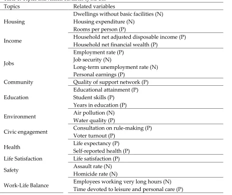
The BLI proposed by OECD in 2011 builds upon Stiglitz et al. (2010)’s claim that the well-being is multidimensional, and, therefore, it should be measured considering simultaneously more than one indicator. The BLI is composed by eleven topics, some of them measured with a single variable and some others measured with a simple average of two or more related variables. The Table 1 describes the composition, in terms of original variables, of each topic.

Table 1: Topics and related variables of the BLI

Topics Related variables

Housing

Dwellings without basic facilities (N) Housing expenditure (N)

Rooms per person (P)

Income Household net adjusted disposable income (P) Household net financial wealth (P)

Jobs

Employment rate (P) Job security (N)

Long-term unemployment rate (N) Personal earnings (P)

Community Quality of support network (P)

Education

Educational attainment (P) Student skills (P)

Years in education (P)

Environment Air pollution (N) Water quality (P)

Civic engagement Consultation on rule-making (P) Voter turnout (P)

Health Life expectancy (P) Self-reported health (P) Life Satisfaction Life satisfaction (P)

Safety Assault rate (N) Homicide rate (N)

Work-Life Balance Employees working very long hours (N) Time devoted to leisure and personal care (P)

4

Online data3 _{originated from the row data have been transformed and aggregated according} to the following procedures: (1) normalization called ‘min max method’(Nardo et al. 2008),

(2) translation applied to negative variables (variables with N in Table 1), and (3) aggregation:

(𝟏) 𝑵𝒐𝒓𝒎 = (_{𝒎𝒂𝒙𝒊𝒎𝒖𝒎 𝒗𝒂𝒍𝒖𝒆 − 𝒎𝒊𝒏𝒊𝒎𝒖𝒎 𝒗𝒂𝒍𝒖𝒆)}𝒐𝒃𝒔𝒆𝒓𝒗𝒆𝒅 𝒗𝒂𝒍𝒖𝒆 − 𝒎𝒊𝒏𝒊𝒎𝒖𝒎 𝒗𝒂𝒍𝒖𝒆 ×𝟏𝟎

(2) 𝐼𝑛𝑑𝑒𝑥 = (1 − 𝑁𝑜𝑟𝑚)

(3) 𝑇𝑜𝑝𝑖𝑐𝑘 = (∑ 𝐼𝑛𝑑𝑒𝑥𝑖 𝑁

𝑖=1

𝑁 ), 𝑘 = 1, … 𝐾

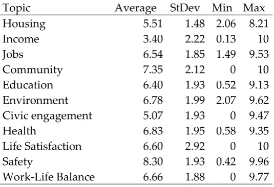
The final database covers 36 Countries over 11 topics. The Table 2Table 2 summarises the descriptive statistics of the scores for each topic.

Table 2. Summary of the topic values

Topic Average StDev Min Max Housing 5.51 1.48 2.06 8.21

Income 3.40 2.22 0.13 10

Jobs 6.54 1.85 1.49 9.53

Community 7.35 2.12 0 10

Education 6.40 1.93 0.52 9.13 Environment 6.78 1.99 2.07 9.62 Civic engagement 5.07 1.93 0 9.47 Health 6.83 1.95 0.58 9.35 Life Satisfaction 6.60 2.92 0 10 Safety 8.30 1.93 0.42 9.96 Work-Life Balance 6.66 1.88 0 9.77 Data extracted on 17 Feb 2016 10:40 UTC (GMT) from OECD.Stat;

As mentioned, for the purpose of our analysis we propose to measure the well-being in terms of the performance according to a bundle of dimensions. Consequently, we proceed to an additional normalization on the topics values:

(4) 𝑁𝑜𝑟𝑚_𝑇𝑜𝑝𝑖𝑐𝑘 = (_∑ 𝑇𝑜𝑝𝑖𝑐_{𝑇𝑜𝑝𝑖𝑐}𝑘 𝑘 𝐾

𝑘=1 ) , 𝑘 = 1, … 𝐾

in order for each country to have the same total amount of BLI. Put differently, since each topic has been further normalised along the cross-section dimension, our distance measure does not depends on the total amount; rather it depends only on the mix of well-being (i.e. the proportions among the topics).

5

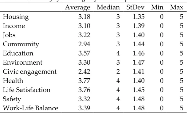
As mentioned, in the dedicate website, people can express their opinion on each topic by rating the topics according to their personal value judgment. The ratings are in a score that is in the interval [0,5]. For each of the person expressing opinion, the website builds its own BLI, with an algorithm that estimates the weighted average of country level values of the topics (performances) multiplied by the subjective scores (value judgments). This algorithm allows the visitors to see in real time how the BLI rank changes with the change in the score associated to the topics. Starting from 2011, more than 100,000 users of the Better Life Index around the world have shared their views and the OECD has collected this data. The microdata can be downloaded and in addition to the individual well-being ratings, they show the territorial origin of the visitors, i.e. the country4_{. We have in total 92,980 individual preferences from all} the 36 Countries where the BLI is measured (we do not consider the preferences from the countries not included in BLI dataset). In Table 3, the descriptive statistics for the weights are reported. Some information, about the perceived trade off, can be seen in the average and median ratings (second and third column in Table 3). On this point ‘Civic engagement’ is, globally, the lowest preferred topic describing the well-being, while ‘Education’, ‘Health’, ‘Life Satisfaction’, and ‘Work-Life Balance’ have the highest average and median values.

Table 3: Summary of the Weights for each Topic

Average Median StDev Min Max

Housing 3.18 3 1.35 0 5

Income 3.10 3 1.39 0 5

Jobs 3.22 3 1.40 0 5

Community 2.94 3 1.44 0 5

Education 3.57 4 1.46 0 5

Environment 3.30 3 1.47 0 5

Civic engagement 2.42 2 1.41 0 5

Health 3.77 4 1.40 0 5

Life Satisfaction 3.76 4 1.45 0 5

Safety 3.32 4 1.48 0 5

Work-Life Balance 3.39 4 1.48 0 5 Data extracted on 17-18 Feb 2016 from OECD.Stat

In order to compare the topic values in (4) with the individual weights, we normalize the topic in the interval [0,5] as the weights. These weights will be used in the measurement of the loss function described in the following section.

3.

The societal loss function

The use of societal loss function stems from the original (unidimensional) spatial model presented in the Hotelling (1929)’s seminal work. Following to Hotelling (1929)’s contribution Downs (1957), for the first time, used a spatial model in a democratic political competition

6

context before Davis et al. (1972) introduced the first multidimensional spatial model to study political competition over multiple policy issues. More precisely, it is worth recalling that in the model proposed by Davis et al. (1972) each policy issue correspond to a dimension in a vector space. The standard approach in political economy is to assume that agents (individuals and policy makers) have an ideal policy represented by a point in the vector space.

Hence, in line with Downs (1957) let us start with a unidimensional policy space, in which the

𝑖-th citizen has a policy preference 𝑔𝑖. According to the 𝑗-th country where she/he lives, the citizen has a disutility proportional to the distance between the policy 𝑔𝑗 implemented in the country 𝑗, and its own preference:

(5) 𝑈𝑖(𝑔𝑗) = −𝑑(𝑔𝑗, 𝑔𝑖)

Following the axiomatic foundation provided in Eguia (2011), in a 𝐾-dimensional policy space the individual disutility on the implemented policy 𝑔𝑗 can be expressed by:

(6) 𝑈𝑖(𝒈𝑗) = −𝑑𝛿(𝒈𝑗, 𝒈𝑖) = (∑|𝑔𝑘𝑗− 𝑔𝑘𝑖| 𝛿 𝐾

𝑘=1

)

1 𝛿 ⁄

The parameter δ represents the agent’s sensitivity to policies different from her preferred mix. To this regard it is worth noticing that while for values of δ≥1 the function (6) is a Minkowski

(1886) metric, with δ<1 the function (5) is not a metric because it violates the triangle inequality (Eguia, 2011). In the extant literature (Kramer, 1977; Enelow, Hinich, 1981; Feddersen, 1992; Schofield, Sened, 2006; Schofield, 2007; Hortala-Vallve, Esteve-Volart, 2011), the preferences on the different policies have been expressed by quadratic utility (distance) function or, more generally, concave in the Euclidean distance to the ideal point of the agent (Eguia, 2011). Consistently with this practice we adopt two different distance functions with δ≥1. Namely, the Euclidean 𝛿 = 2 and the taxicab 𝛿 = 1.

In order to aggregate the individual loss function at country level, a decision must be taken about the social welfare function. On the point two extreme views have been proposed: the Bentham Utilitarianism (Bentham, 1789), and the Rawlsian (Rawls, 1971). According to the Benthamian approach the social welfare function is given by the sum of the individual utilities. Therefore, the function conceptually accepts a complete trade-off (or compensability) among individual utilities. In our case, for the country 𝑗 the societal loss function for the implemented policy 𝑔𝑗 is:

(7) 𝑈𝑗𝐵(𝑔𝑗) = ∑ 𝑈𝑖(𝑔𝑗)

𝑖 = ∑ −𝑑(𝒈 𝑗_{, 𝒈}𝑖₎ 𝑖

7

of different election methods. Since we have a differentiated dataset where the number of voters changes among the different countries, we propose to measure the Bentham country-level disutility as the average loss function (average loss per preference):

(8) 𝑈_𝑗𝐵_(𝒈𝑗_{) =}1

𝑛 ∑ 𝑈_𝑖 𝑖(𝒈𝑗)=1_{𝑛 ∑ −𝑑(𝒈}𝑗, 𝒈𝑖)

𝑖

where 𝑛 is the number of voters in the country 𝑗.

In the Rawlsian approach instead, the social utility function is given by the minimum of the individual utilities. In our case, therefore, for the country 𝑗 the societal loss function for the implemented policy 𝑔𝑗 is equal to the maximum value achieved by the distance function:

(9) 𝑈_𝑗𝑅_(𝒈𝑗_{) = min} 𝑖=1,…,𝑛𝑈𝑖(𝒈

𝑗_{) = max} 𝑖=1,…,𝑛𝑑(𝒈

𝑗_{, 𝒈}𝑖₎

where 𝑈_𝑗𝑅(𝒈) is the Rawlsian societal disutility for the policy 𝒈𝑗, and 𝑈_𝑖(𝒈𝑗) are the individual disutilities as proposed in (6). In other words, the Rawls country-level disutility is given by the disutility of the less happy citizen (maxi-min method).

The following section presents an analysis of the societal loss of well-being according to both the Benthamian and the Rawlsian approach.

An alternative new way to measure the well-being on BLI at country-level, is treating all the individuals as a unique global community and evaluating the policy makers’ offer in terms of mix of well-being, on the basis of the global societal favourite country. Denoting by 𝑔𝑗 the mix of well-being in the country 𝑗 (𝑗 = 1, . . , 𝑚), then for the individual 𝑖, the favourite country in the set is the country that minimizes her loss function:

(10) _{𝑗=1,…,𝑚}max 𝑈𝑖(𝑔𝑗) = min_{𝑗=1,…,𝑚}𝑑𝛿(𝑔𝑗, 𝑔𝑖) = min_{𝑗=1,..,𝑚}(∑|𝑔𝑘𝑗− 𝑔𝑘𝑖| 𝛿 𝐾

𝑘=1

)

1 𝛿 ⁄

Moreover, we can find the least favourite country for the individual 𝑖, as the country that maximizes her loss function:

(11) _{𝑗=1,…,𝑚}min 𝑈𝑖(𝑔𝑗) = max_{𝑗=1,…,𝑚}𝑑𝛿(𝑔𝑗, 𝑔𝑖) = max_{𝑗=1,…,𝑚}(∑|𝑔𝑘𝑗− 𝑔𝑘𝑖| 𝛿 𝐾

𝑘=1

)

1 𝛿 ⁄

By adopting such a global lens, we can evaluate the countries on the basis of the share of people that ranks the country first and last.

4.

Results

8

Euclidean distance, and (ii) the taxicab norm. Moreover, we express the societal loss of well-being with two different aggregations of individual loss functions: the Benthamian societal welfare function (eq. 8), and the Rawlsian social welfare function (eq. 9). As a result of the combination between distance function and aggregate social loss we obtain four different values of social loss for each country. These results are reported in Section 4.1; then, in Section 4.2, we contrast the above loss values with three different indicators of ‘voice’ taken from the World Happiness Indicator (Helliwell et al. 2016), and from the Worldwide Governance Indicators (Kaufmann et al. 2011). Furthermore, in Section 4.3 we compare our loss function with different composite indices of well-being from BLI; and finally (in Section 4.4) we to compare the country level BLI by minimizing the individual loss functions.

4.1. The societal loss of Better Life Index

As mentioned, in this section four societal loss functions are presented: 1. the individual taxicab aggregated with the Benthamian approach, 2. the individual taxicab aggregated with the Rawlsian approach, 3. the individual Euclidean aggregated with the Benthamian approach, and 4. the individual Euclidean aggregated with the Rawlsian approach. Table 4 reports the country-level societal loss5 _{due to mismatching between the individually optimal} mix of well-being and the mix of well-being provided by the policy makers at country level. It is worth noticing that the highest societal loss is registered in Turkey regardless of both the functional forms and the aggregation techniques. The aggregation technique, however, plays a role in determining the second highest societal loss. With both taxicab and Euclidean individual distance function while the second highest loss is achieved by Mexico according to the Benthamian aggregation, the same rank is achieved by Brazil according to the Rawlsian aggregation. On the bottom side of the rank (i.e. better performance due to lower loss values) is placed Norway when using the Bentham aggregation and Finland when using the Rawlsian approach.

Table 4. Societal Loss of BLI

country taxicab norm Euclidean Bentham Rawls Bentham Rawls Australia 20.21 35 7.33 11.18 Austria 18.30 33 6.48 10.44 Belgium 20.03 34 7.26 11.05 Brazil 24.61 45 9.10 14.46 Canada 17.36 38 6.50 11.83

5 _{As long as the form of the individual loss function is concerned, we do not observe relevant differences}

9

Chile 22.51 39 8.53 13.23

Czech Republic 21.88 34 7.91 11.75 Denmark 18.63 34 6.85 10.86 Estonia 23.72 41 8.74 13.53 Finland 17.44 32 6.47 10.25 France 17.46 36 6.54 11.49 Germany 17.24 34 6.41 10.95 Greece 22.39 35 8.38 12.37 Hungary 23.02 36 8.47 12.29 Iceland 20.66 35 7.73 11.79 Ireland 19.23 35 6.87 11.18 Israel 19.83 36 7.38 12.00

Italy 22.13 39 8.19 12.21

Japan 20.55 33 7.67 10.82

Korea 24.00 36 8.73 12.25

Luxembourg 21.77 33 7.78 10.82 Mexico 26.81 39 9.73 13.56 Netherlands 19.59 35 7.35 11.62 New Zealand 18.83 32 6.84 10.39 Norway 16.79 33 6.23 10.44 Poland 26.10 41 9.30 13.15 Portugal 21.50 33 8.03 11.45 Russia 25.17 45 9.01 14.39 Slovak Republic 23.17 34 8.52 11.58 Slovenia 16.96 34 6.39 10.86

Spain 21.88 40 8.14 13.11

Sweden 20.70 33 7.46 10.77 Switzerland 20.87 35 7.58 11.62 Turkey 27.53 46 9.99 14.83 United Kingdom 18.72 34 6.69 10.68 United States 23.59 43 8.37 13.38

Source: authors’ analysis on data from OECD.

An extensive discussion of the loss and of the related ranking achieved by each country goes beyond the scope of the current analysis. Nonetheless, in what follows we conjecture that the ‘voice’ aspect of the democratic processes ongoing in the considered countries can positively influence the way the final observed outcome in terms of mix of well-being indicators reflects citizens’ preferences on the same matter. Next section addresses this issue.

4.2. Comparisons among different indexes of ‘voice’

10

for another policy maker, by a revolution, or by changing country (Hirschman, 1970). Therefore, the differences in the mismatching between individual and country-level mix can be explained by the balance of the operating of these forces. In this section we explore to what extent the mismatching between the individual optimal mix and the policy maker mix can be explained in terms lack of involvement of citizens in the decisions.

To this end we show the relation between our societal loss function and some proxies of quality of democracy provided by the international institutions. We choose three different indicators to measure the quality of the democracy: the index of ‘Freedom to make life choices’, and the index of ‘Democratic Quality’, both provided by World Happiness Index (Helliwell et al. 2016); and the ‘Voice Index’ provided by the Worldwide Governance Indicators (Kaufmann et a. 2011). Table A1 in the Appendices shows that there is significant negative correlation between our estimated loss functions and any voice index taken into account. Indeed, the correlation between the index of ‘Freedom to make life choices’ and our loss function is -0.53, -0.58, -0.35, and -0.51, using respectively taxicab Bentham, Euclidean Bentham, taxicab Rawls, and Euclidean Rawls. The correlation between the index of ‘Democratic Quality’ and our loss function is -0.66, -0.68, -0.70, -0.77, using respectively taxicab Bentham, Euclidean Bentham, taxicab Rawls, and Euclidean Rawls. The correlation between the ‘Voice Index’ is -0.72, -0.74, -0.57, -0.66, using respectively taxicab Bentham, Euclidean Bentham, taxicab Rawls, and Euclidean Rawls. These results reveal that there is a strong relation between our societal loss function and the lack in the quality of the democracy. This proves that our approach can be considered as a valuable support to understand social phenomena and the OECD survey is quite representative.

Since the correlation between the taxicab and the Euclidean preferences is close to one (see Table A1 in the Appendices), for convenience of presentation we are going to use only the taxicab preferences in this stage of the analysis.

We propose a quadrant analysis in order to explore similarities among countries with similar level of loss function and voice indices. Figure 1 shows the relation between the estimated loss

functions and the index of ‘Freedom to make life choices’ (Helliwell et al., 2016). Figures 1, 2, 3, 4, and 5 report two lines representing the respective average values. Since the correlation between the two variable is negative (Tab. A1 in the Appendices), the majority of values lay on the second and the fourth quadrant. In other words, countries with more (less) societal loss function have also less (more) freedom to make life choices. There are some interesting exceptions in Figure 1: Israel has less freedom to make life choice, and it has also lower values of societal loss function. On the other side, USA, and Poland have high freedom to make life choice and quite interestingly also high societal loss function. These evidences may signal that in these countries other factors (not included in the BLI) play a relevant rule in the individuals’

11

Figure 1

relation between the societal loss functions of BLI and ‘

(The cross represents the average values)

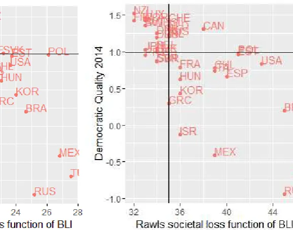
Figure 2Figure 2 shows the relation between the estimated loss functions and the index of ‘Democratic Quality’ (Helliwell et al. 2016). Alike the previous case, due to the negative correlations between these variables (Tab. A1 in the Appendices), the values tend to concentrate into the second and the fourth quadrant. It is worth noticing the presence of some outliers such as, again, Israel that have low democratic quality and also low societal loss of being and Canada showing high democratic quality and high Rawls societal loss of well-being.

12

Figure 3Figure 3 shows the relation between the estimated loss functions and the ‘Voice Index’

(

). In terms of robustness, it is worth noticing that although the

‘Voice Index’

is estimated by another institution, we observe that the big picture is quite

close to that of Figure 1 and Figure 2. We observe the majority of the values on the

second and fourth quadrant and almost the same interesting outliers: Israel, Canada,

and USA.

Figure 3 relation between the societal loss functions of BLI and

‘

’

4.3. The relation between loss function and composite indices of well-being from BLI

13

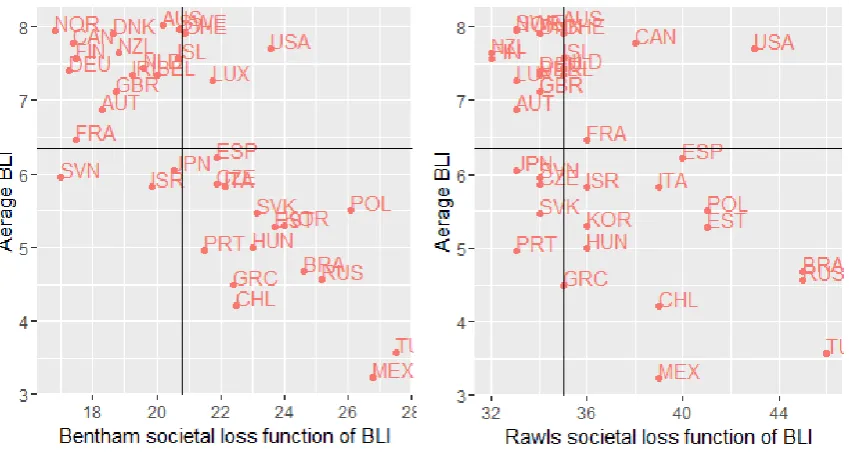
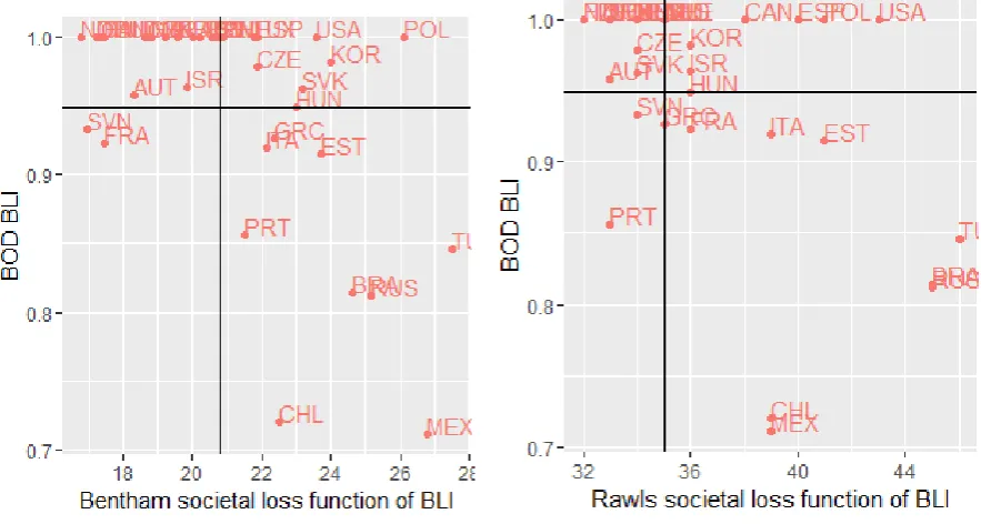
most interesting cases are USA and Canada with both a high average well-being and a high societal loss function. In this case, therefore, we have a high level of well-being that is not matching with people preferences as expressed in the BLI. On the other side, we observe that in Portugal, despite the lower amount of well-being, the Rawlsian loss function is low.

Figure 4 relation between the societal loss functions of BLI and the average BLI

’

14

Figure 5 relation between the societal loss functions of BLI and the BOD BLI

’

4.4. The country-level loss function

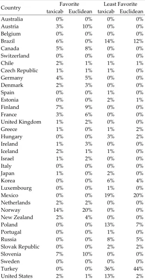
This section introduces a new way to measure the well-being on BLI at country-level. One that (i) treats all the individuals as a unique global community and (ii) evaluate the policy makers’ offer in terms of mix of well-being, on the basis of the global societal favourite country. The underlying idea is that each individual has its own favourite country according to the distance between its optimal point and the country-level mix. Formally, for each individual the favourite country is the country that minimizes her loss function (10), and the least favourite country is the country that maximizes her loss function (11). By adopting such a global lens, we evaluate the countries on the basis of the share of people that ranks the country first and last.

Table 5 shows the share of 92,968 individuals belonging to the sample collected from the OECD website that ranks each country first and last with taxicab and Euclidean loss function. On the top side of the rank (second and third column in Table 5) Norway is the favoured Country according to the majority of individuals. This result is substantially confirmed with both taxicab and Euclidean loss function. Indeed, the 14% of individuals ranks Norway first assuming taxicab loss function, and the 20% of individuals ranks Norway first assuming Euclidean loss function. Finland and Slovenia register a relatively good ranking placing them among the first three countries assuming taxicab loss function. Similarly, Austria and Slovenia are placed among the first three countries according to the Euclidean loss function.

15

respectively. In the last third positions, there are also Mexico and Brazil, both with the taxicab and Euclidean loss function.

Table 5 Share of individuals ranking the country first and last

Country Favorite Least Favorite taxicab Euclidean taxicab Euclidean

Australia 0% 0% 0% 0%

Austria 3% 10% 0% 0%

Belgium 0% 0% 0% 0%

Brazil 6% 0% 14% 12%

Canada 5% 8% 0% 0%

Switzerland 0% 0% 0% 0%

Chile 2% 1% 1% 1%

Czech Republic 1% 1% 1% 0%

Germany 4% 5% 0% 0%

Denmark 2% 3% 0% 0%

Spain 0% 0% 1% 0%

Estonia 0% 0% 2% 1%

Finland 7% 9% 0% 0%

France 3% 6% 0% 0%

United Kingdom 1% 2% 0% 0%

Greece 1% 0% 1% 2%

Hungary 0% 0% 3% 2%

Ireland 1% 3% 0% 0%

Iceland 2% 1% 1% 0%

Israel 1% 2% 0% 0%

Italy 0% 0% 0% 0%

Japan 1% 0% 2% 0%

Korea 0% 0% 6% 4%

Luxembourg 0% 0% 1% 0%

Mexico 0% 0% 19% 20%

Netherlands 2% 2% 0% 0%

Norway 14% 20% 0% 0%

New Zealand 2% 4% 0% 0%

Poland 0% 0% 13% 7%

Portugal 0% 0% 1% 0%

Russia 0% 0% 8% 5%

Slovak Republic 0% 0% 2% 2%

Slovenia 7% 10% 0% 0%

Sweden 0% 0% 0% 0%

Turkey 0% 0% 36% 44%

16

5.

Conclusions

This paper addressed the issue of whether and to what extent real people’s preferences among different dimensions of a multidimensional measure of well-being match with the wellbeing mix effectively registered in the OECD countries as captured by the Better Life Index framework. The OECD BLI is particularly suitable for this kind of analysis because it is one of the largest dataset collecting well-being data at country level. Moreover, OECD provides a survey of the user weightings related to 11 different topics. By using these data, we interpret the country-level citizens’ individual weightings as the optimal subjective mix of well-being, and we interpret the country-level values of the topics as the mix of well-being provided by policy makers. According to these assumptions, we assess the societal loss of well-being at country-level by estimating the distance between these mixes for each country included in the OECD survey.

To the best of our knowledge, for the first time, a multidimensional spatial model of preferences is used in the well-being context. In our model, the OECD countries are objects of preferences. These preferences are expressed as points in the Euclidean K-dimensional space in which each dimension is a specific aspect of well-being. Each individual/voter is characterized by her/his ideal point in the aforementioned space. Then, for each individual, the distance between its optimal mix of well-being and the mix provided by policy makers can be interpreted as individual loss in well-being. Therefore, the countries are judged as good as they are close to the voters’ ideal point.

The main results based on the novel methodology are that the highest societal losses are registered in Turkey, Mexico, and Brazil. While the lowest societal losses are in Norway and in Finland. By comparing our estimated societal losses and some proxies of ‘voice’ provided by different source of data (Helliwell et al. 2016, Kaufmann et al. 2011), it emerges that countries with lower levels democracy are also countries with higher levels of societal loss of well-being. Therefore, the detected mismatching between will of the people and policy makers’ activity may be due to lack of citizens’ involvement in the decisions making process. Moreover, by comparing the societal loss function and the BLI it emerges that countries with more mismatching are also countries with less Better Life Index.

Appendices

Table A1, Rank Correlation Matrix with confidence intervals (95 % bootstrap upper and lower bounds)

A B C D E F G H I L

A 1

LB 0.982

B 0.991 1

17 LB 0.504 0.508

C 0.714 0.717 1

UB 0.845 0.846

LB 0.700 0.736 0.899

D 0.836 0.857 0.948 1 UB 0.914 0.925 0.973

LB -0.732 -0.765 -0.611 -0.721

E -0.531 -0.582 -0.353 -0.514 1 UB -0.246 -0.314 -0.028 -0.223

LB -0.813 -0.822 -0.835 -0.876 0.364

F -0.661 -0.676 -0.698 -0.769 0.619 1 UB -0.425 -0.446 -0.480 -0.589 0.787

LB -0.721 -0.743 -0.570 -0.657 0.504 0.185

G -0.515 -0.548 -0.297 -0.419 0.714 0.484 1 UB -0.224 -0.267 0.035 -0.105 0.845 0.701

LB -0.852 -0.857 -0.830 -0.874 0.294 0.840 0.211

H -0.726 -0.736 -0.689 -0.766 0.568 0.916 0.505 1 UB -0.523 -0.538 -0.466 -0.585 0.755 0.956 0.715

LB -0.741 -0.769 -0.731 -0.802 0.086 0.447 0.029 0.457 I -0.544 -0.590 -0.529 -0.643 0.403 0.676 0.354 0.683 1 UB -0.263 -0.324 -0.243 -0.399 0.646 0.822 0.612 0.826 LB -0.856 -0.883 -0.741 -0.846 0.537 0.628 0.534 0.685 0.658 L -0.734 -0.781 -0.546 -0.717 0.736 0.793 0.734 0.828 0.811 1 UB -0.535 -0.608 -0.265 -0.509 0.857 0.890 0.856 0.909 0.900 Bootstrap with 1000 replicates, using R package by Herve´ (2015)

Note: LB=Lower Bound, UB =Upper Bond, A=taxicab Bentham, B=Euclidean Bentham, C=taxicab Rawls, D=Euclidean Rawls, E= Freedom to make life choices 2008-2015, F= Democratic Quality 2008-2014, G=World Happiness Index 2016, H= Voice Index WB, I=BOD BLI, L=Average BLI

References

Bentham, J. (1789). An Introduction to the Principles of Morals and Legislation (Payne, London). Reprinted in 1970 in: J.M. Burns and H.L.A. Hart, eds. (Athlone Press, London).

Bleys, B. (2012). Beyond GDP: Classifying Alternative Measures for Progress, Social Indicators Research, 109, 355–376.

18

Costanza, R., Daly, L., Fioramonti, L., Giovannini, E., Kubiszewski, I., Mortensen, L. F., ... & Wilkinson, R. (2016). Modelling and measuring sustainable wellbeing in connection with the UN Sustainable Development Goals. Ecological Economics, 130, 350-355.

Costanza, R., Kubiszewski, I., Giovannini, E., Lovins, H., McGlade, J., Pickett, K. E., ... & Wilkinson, R. (2014). Development. Nature, 505(7483), 283-285.

Coyle D. (2014) GDP: A brief but affectionate history, Princeton University Press, Princeton.

Davis, O. A., DeGroot, M. H., & Hinich, M. J. (1972). Social preference orderings and majority rule. Econometrica: Journal of the Econometric Society, 147-157.

De Beukelaer C. (2014) Gross Domestic Problem: The Politics Behind the World's Most Powerful Number, Journal of Human Development and Capabilities 15.2-3, 290-291.

Downs, A. (1957). An economic theory of political action in a democracy. Journal of Political Economy, 65(2), 135-150.

Eguia, J. X. (2011). Foundations of spatial preferences. Journal of Mathematical Economics, 47(2), 200-205.

Enelow, J., & Hinich, M. J. (1981). A new approach to voter uncertainty in the Downsian spatial model. American journal of political science, 483-493.

Feddersen, T. J. (1992). A voting model implying Duverger's law and positive turnout.

American journal of political science, 938-962.

Fioramonti L. (2013) Gross domestic problem: The politics behind the world's most powerful number, Zed Books.

Fleurbaey M. (2009) Beyond GDP: The quest for a measure of social welfare, Journal of Economic Literature, 1029-1075

Frey, B. S., & Stutzer, A. (2010). Happiness and public choice. Public Choice, 144(3-4), 557-573.

Helliwell, J. F., Huang, H., & Wang, S. (2016). The distribution of world happiness. WORLD HAPPINESS, 8.

Herve´, M. (2015). RVAideMemoire: Diverse basic statistical and graphical functions, R package version 0.9-52. http://CRAN.R-project.org/package=RVAideMemoire.

Hirschman A.O. (1970) Exit, voice, and loyalty: Responses to decline in firms, organizations, and states (Vol. 25). Harvard university press.

19

Hotelling, H. (1929). Stability in competition. Economic Journal, 39 (153), 41-57.

Karabell Z. (2014) The leading indicators: a short history of the numbers that rule our world, Simon and Schuster.

Kaufmann, D., Kraay, A., & Mastruzzi, M. (2011). The worldwide governance indicators: methodology and analytical issues. Hague Journal on the Rule of Law, 3(2), 220-246.

Kramer, G. H. (1977). A dynamical model of political equilibrium. Journal of Economic Theory, 16(2), 310-334.

Minkowski, H. (1886). Geometrie der Zahlen. Teubner Verlag, Leipzig.

Mizobuchi, H. (2014). Measuring world better life frontier: a composite indicator for

OECD better life index.

Social Indicators Research

,

118

(3), 987-1007.

OECD. (2011). Compendium of Oecd well-being indicators. Paris: OECD Publishing.

Patrizii, V., Pettini, A., & Resce, G. (2017). The Cost of Well-Being. Social Indicators Research,

133(3), 985-1010.

Rawls, J. (1971). A Theory of Justice, Harvard University Press, Cambridge, Mass.

Schofield, N. (2007). The mean voter theorem: necessary and sufficient conditions for convergent equilibrium. The Review of Economic Studies, 74(3), 965-980.

Schofield, N., & Sened, I. (2006). Multiparty democracy: elections and legislative politics.

Cambridge University Press.

Smith, W. D. (2000). Range voting. The paper can be downloaded from the author’s homepage at

http://www. math. temple. edu/~ wds/homepage/works. html.

Stiglitz, J. E., Sen, A., & Fitoussi, J. P. (2010). Report by the commission on the measurement of economic performance and social progress. Paris: Commission on the Measurement of Economic Performance and Social Progress.

Tiebout, C. M. (1956). A pure theory of local expenditures. Journal of political economy, 64(5), 416-424.

UNDP (1996) Human Development Report. United Nation Development Programme, Nairobi, Kenia.