Proceedings of the BioNLP 2019 workshop, pages 298–308 298
Embedding Biomedical Ontologies by Jointly Encoding
Network Structure and Textual Node Descriptors
Sotiris Kotitsas1, Dimitris Pappas1,2, Ion Androutsopoulos1, Ryan McDonald1,3 and Marianna Apidianaki4
1Department of Informatics, Athens University of Economics and Business, Greece
2Institute for Language and Speech Processing, Research Center ‘Athena’, Greece
3Google Research
4CNRS, LLF, Univ. Paris Diderot, France
{p3150077, pappasd, ion}@aueb.gr [email protected], [email protected]
Abstract
Network Embedding (NE) methods, which map network nodes to low-dimensional fea-ture vectors, have wide applications in net-work analysis and bioinformatics. Many ex-istingNEmethods rely only on network struc-ture, overlooking other information associated with the nodes, e.g., text describing the nodes. Recent attempts to combine the two sources of information only consider local network struc-ture. We extendNODE2VEC, a well-knownNE
method that considers broader network struc-ture, to also consider textual node descriptors using recurrent neural encoders. Our method is evaluated on link prediction in two net-works derived fromUMLS. Experimental re-sults demonstrate the effectiveness of the pro-posed approach compared to previous work.
1 Introduction
Network Embedding (NE) methods map each node of a network to an embedding, meaning a low-dimensional feature vector. They are highly effective in network analysis tasks involving pre-dictions over nodes and edges, for example link prediction (Lu and Zhou,2010), and node classi-fication (Sen et al.,2008).
EarlyNEmethods, such asDEEPWALK(Perozzi
et al.,2014),LINE(Tang et al.,2015),NODE2VEC
(Grover and Leskovec, 2016), GCNs (Kipf and
Welling, 2016), leverage information from the
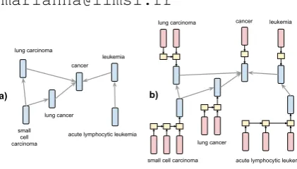
network structure to produce embeddings that can reconstruct node neighborhoods. The main advan-tage of these structure-oriented methods is that they encode the network context of the nodes, which can be very informative. The downside is that they typically treat each node as an atomic unit, directly mapped to an embedding in a look-up table (Fig. 1a). There is no attempt to model information other than the network structure, such
lung cancer cancer lung carcinoma leukemia
small cell carcinoma lung cancer
cancer
acute lymphocytic leukemia lung carcinoma
leukemia
small cell carcinoma
a) b)
[image:1.595.309.520.219.339.2]acute lymphocytic leukemia
Figure 1: Example network with nodes associated with textual descriptors. a) A model where each node is rep-resented by a vector (node embedding) from a look-up table. b) A model where each node embedding is gen-erated compositionally from the word embeddings of its descriptor via anRNN. The latter model can learn node embeddings from both the network structure and the word sequences of the textual descriptors.
as textual descriptors (labels) or other meta-data associated with the nodes.
More recentNEmethods, e.g.,CANE(Tu et al.,
2017),WANE(Shen et al.,2018), produce
embed-dings by combining the network structure and the text associated with the nodes. These content-oriented methods embed networks whose nodes are rich textual objects (often whole documents). They aim to capture the compositionality and se-mantic similarities in the text, encoding them with deep learning methods. This approach is illus-trated in Fig. 1b. However, previous methods of this kind considered impoverished network con-texts when embedding nodes, usually single-edge hops, as opposed to the non-local structure con-sidered by most structure-oriented methods.
a NE method only needs to model the role of ‘acute’ as a modifier that can be included in the de-scriptor of a node (e.g., a disease node) to specify a sub-type. This property can be learned (and en-coded in the word embedding of ‘acute’) if several similar IS-A edges, with ‘acute’ being the only extra word in the descriptor of the sub-type, ex-ist in the network. This strategy would not how-ever be successful in ‘p53’ (a protein)IS-A‘tumor suppressor’, where no word in the descriptors fre-quently denotes sub-typing. Instead, by consider-ing the broader network context of the nodes (i.e. longer paths that connect them), aNEmethod can detect that the two nodes have common neighbors and, hence, adjust the two node embeddings (and the word embeddings of their descriptors) to be close in the representation space, making it more likely to predict anIS-Arelation between them.
We propose a newNEmethod that leverages the strengths of both structure and content-oriented approaches. To exploit wide network contexts, we follow NODE2VEC(Grover and Leskovec, 2016) and generate random walks to construct the net-work neighborhood of each node. The SKIP -GRAM model (Mikolov et al., 2013) is then used to learn node embeddings that successfully pre-dict the nodes in each walk, from the node at the beginning of the walk. To enrich the node em-beddings with information from their textual de-scriptors, we replace the NODE2VEC look-up ta-ble with various architectures that operate on the word embeddings of the descriptors. These in-clude simply averaging the word embeddings of a descriptor, and applying recurrent deep learning encoders. The proposed method can be seen as an extension ofNODE2VECthat incorporates textual node descriptors. We evaluate several variants of the proposed method on link prediction, a stan-dard evaluation task forNEmethods. We use two biomedical networks extracted from UMLS (
Bo-denreider, 2004), with PART-OF and IS-A
rela-tions, respectively. Our method outperforms sev-eral existing structure and content-oriented meth-ods on both datasets. We make our datasets and source code available.1
2 Related work
Network Embedding (NE) methods, a type of rep-resentation learning, are highly effective in
net-1https://github.com/SotirisKot/
Content-Aware-N2V
work analysis tasks involving predictions over nodes and edges. Link prediction has been ex-tensively studied in social networks (Wang et al.,
2015), and is particularly relevant to bioinfor-matics where it can help, for example, to dis-cover interactions between proteins, diseases, and genes (Lei and Ruan,2013;Shojaie,2013;Grover
and Leskovec, 2016). Node classification can
also help analyze large networks by automati-cally assigning roles or labels to nodes (Ahmed
et al., 2018; Sen et al., 2008). In
bioinformat-ics, this approach has been used to identify pro-teins whose mutations are linked with particular diseases (Agrawal et al.,2018).
A typical structure-oriented NE method is DEEPWALK (Perozzi et al., 2014), which learns node embeddings by applying WORD2VEC’s SKIPGRAMmodel (Mikolov et al.,2013) to node sequences generated via random walks on the network. NODE2VEC (Grover and Leskovec,
2016) explores different strategies to perform ran-dom walks, introducing hyper-parameters to guide them and generate more flexible neighborhoods.
LINE(Tang et al.,2015) learns node embeddings
by exploiting first- and second-order proximity in-formation in the network. Wang et al. (2016) learn node embeddings that preserve the proxim-ity between 2-hop neighbors using a deep autoen-coder. Yu et al. (2018) encode node sequences generated via random walks, by mapping the walks to low dimensional embeddings, through an LSTMautoencoder. To avoid overfitting, they use a generative adversarial training process as regu-larization. Graph Convolutional Networks (GCNs) are a graph encoding framework that also falls within this paradigm (Kipf and Welling, 2016;
Schlichtkrull et al., 2018). Unlike other
meth-ods that use random walks or static neighbour-hoods, GCNs use iterative neighbourhood averag-ing strategies to account for non-local graph struc-ture. All the aforementioned methods only encode the structural information into node embeddings, ignoring textual or other information that can be associated with the nodes of the network.
Previous work on biomedical ontologies (e.g., Gene Ontology, GO) suggested that their terms, which are represented through textual descriptors, have compositional structure. By modeling it, we can create richer representations of the data en-coded in the ontologies (Mungall, 2004; Ogren
the argument of compositionality by observing that manyGOterms contain otherGOterms. Also, they argue that substrings that are not GO terms appear frequently and often indicate semantic re-lationships. Ogren et al. (2004) use finite state automata to representGO terms and demonstrate how small conceptual changes can create biologi-cally meaningful candidate terms.
In other work onNEmethods,CENE(Sun et al.,
2016) treats textual descriptors as a special kind of node, and uses bidirectional recurrent neural net-works (RNNs) to encode them. CANE (Tu et al.,
2017) learns two embeddings per node, a text-based one and an embedding text-based on network structure. The text-based one changes when inter-acting with different neighbors, using a mutual at-tention mechanism.WANE(Shen et al.,2018) also uses two types of node embeddings, text-based and structure-based. For the text-based embed-dings, it matches important words across the tex-tual descriptors of different nodes, and aggregates the resulting alignment features. In spite of per-formance improvements over structure-oriented approaches, these content-aware methods do not thoroughly explore the network structure, since they consider only direct neighbors.
By contrast, we utilize NODE2VEC to obtain wider network neighborhoods via random walks, a typical approach of structure-oriented methods, but we also use RNNs to encode the textual de-scriptors, as in some content-oriented approaches. Unlike CENE, however, we do not treat texts as separate nodes; unlikeCANE, we do not learn sep-arate embeddings from texts and network struc-ture; and unlike WANE, we do not align the de-scriptors of different nodes. We generate the em-bedding of each node from the word emem-beddings of its descriptor via theRNN (Fig.1), but the pa-rameters of theRNN, the word embeddings, hence also the node embeddings are updated during training to predictNODE2VEC’s neighborhoods.
Although we use NODE2VEC to incorporate network context in the node embeddings, other neighborhood embedding methods, such asGCNs, could easily be used too. Similarly, text encoders other than RNNs could be applied. For
exam-ple,Mishra et al.(2019) try to detect abusive
lan-guage in tweets with a semi-supervised learning approach based on GCNs. They exploit the net-work structure and also the labels associated with the tweets, taking into account the linguistic
be-havior of the authors.
3 Proposed Node Embedding Approach
Consider a network (graph)G=hV, E, Si, where V is the set of nodes (vertices); E ⊆ V ×V is the set of edges (links) between nodes; andSis a function that maps each nodev∈V to its textual descriptor S(v) = hw1, w2, . . . , wni, where nis
the word length of the descriptor, and each word wicomes from a vocabularyW. We consider only
undirected, unweighted networks, where all edges represent instances of the same (single) relation-ship (e.g.,IS-AorPART-OF). Our approach, how-ever, can be extended to directed weighted net-works with multiple relationship types. We learn an embedding f(v) ∈ Rd for each node v ∈ V.
As a side effect, we also learn a word embedding e(w)for each vocabulary wordw∈W.
To incorporate structural information into the node embeddings, we maximize the predicted
probabilitiesp(u|v)of observing theactual neigh-bors u ∈ N(v) of each ‘focus’ node v ∈ V, whereN(v)is the neighborhood ofv, andp(u|v)
is predicted from the node embeddings ofu and v. The neighbors N(v) ofv are not necessarily directly connected to v. In real-world networks, especially biomedical, many nodes have few di-rect neighbors. We use NODE2VEC(Grover and
Leskovec, 2016) to obtain a larger neighborhood
for each nodev, by generating random walks from v. For every focus nodev∈V, we computer ran-dom walks (paths) Pv,i = hvi,1 =v, vi,2, ..., vi,ki
(i = 1, . . . , r) of fixed lengthk through the net-work (vi,j ∈ V).2 The predicted probability
p(vi,j = u) of observing node u at step j of
a walk Pv,i that starts at focus node v is taken
to depend only on the embeddings of u, v, i.e., p(vi,j =u) =p(u|v), and can be estimated with
a softmax as in the SKIPGRAM model (Mikolov
et al.,2013):
p(u|v) = exp(f
0(u)·f(v))
P
u0∈V exp(f0(u0)·f(v))
(1)
where it is assumed that each nodevhas two dif-ferent node embeddings, f(v), f0(v), used when
2
Our networks are unweighted, hence we use uniform edge weighting to traverse them.NODE2VEChas two hyper-parameters,p, q, to control the locality of the walk. We set
p=q= 1(default values). For efficiency,NODE2VEC actu-ally performsrrandom walks of lengthl≥k; then it usesr
v is the focus node or the predicted neigh-bor, respectively, and · denotes the dot prod-uct. NODE2VEC minimizes the following objec-tive function:
L=−X v∈V
r
X
i=1
k
X
j=2
logp(vi,j|vi,1=v) (2)
in effect maximizing the likelihood of observing the actual neighbors vi,j of each focus node v
that are encountered during the r walks Pv,i = hvi,1 =v, vi,2, ..., vi,ki(i= 1, . . . , r) fromv.
Cal-culating p(u|v) using a softmax (Eq. 1) is com-putationally inefficient. We apply negative sam-pling instead, as in WORD2VEC (Mikolov et al.,
2013). Thus, NODE2VEC is analogous to SKIP -GRAM WORD2VEC, but using random walks from each focus node, instead of using a context win-dow around each focus word in a corpus.
As already mentioned, the originalNODE2VEC does not consider the textual descriptors of the nodes. It treats each node embedding f(v) as a vector representing an atomic unit, the node v; a look-up table directly maps each node v to its embedding f(v). This does not take advantage of the flexibility and richness of natural language (e.g., synonyms, paraphrases), nor of its composi-tional nature. To address this limitation, we sub-stitute the look-up table whereNODE2VECstores the embeddingf(v) of each node v with a neu-ral sequence encoder that producesf(v)from the word embeddings of the descriptorS(v)ofv.
More formally, let every wordw∈W have two embeddingse(w)ande0(w), used whenwoccurs in the descriptor of a focus node, and whenw oc-curs in the descriptor of a neighbor of a focus node (in a random walk), respectively. For every node v ∈ V with descriptorS(v) = (w1, . . . , wn), we
create the sequencesT(v) = he(w1), . . . , e(wn)i
andT0(v) = he0(w1), . . . , e0(wn)i. We then set
f(v) = ENC(T(v)) and f0(v) = ENC(T0(v)), where ENC is the sequence encoder. We outline below three specific possibilities forENC, though it can be any neural text encoder. Note that the embeddings f(v) and f0(v) of each node v are constructed from the word embeddingsT(v)and T0(v), respectively, of its descriptor S(v) by the encoder ENC. The word embeddings of the de-scriptor and the parameters ofENC, however, are also optimized during back-propagation, so that the resulting node embeddings will predict (Eq.1) the actual neighbors of each focus node (Fig.2).
right twelfth rib body of right twelfth rib external surface of right twelfth rib
focus node predicted neighbor
Encoder Encoder Encoder
f'(v1) f(v2) f'(v3)
optimize optimize
[image:4.595.314.516.71.156.2]predicted neighbor
Figure 2: Illustration of the proposedNEapproach.
For simplicity, we only mention f(v) and T(v)
below, but the same applies tof0(v)andT0(v).
AVG-N2V: For every node v ∈ V, this model constructs the node’s embedding f(v) by sim-ply averaging the word embeddings T(v) =
he(w1), . . . , e(wn)iofS(v) = (w1, w2, . . . , wn).
f(v) = 1
n
n
X
i=1
e(wi) (3)
GRU-N2V: Although averaging word embeddings is effective in text categorization (Joulin et al.,
2016), it ignores word order. To account for or-der, we apply RNNs with GRU cells (Cho et al.,
2014) instead. For each node v ∈ V with de-scriptorS(v) = hw1, . . . , wni, this method
com-putesnhidden state vectorsH =hh1, . . . , hni=
GRU(e(w1), . . . , e(wn)). The last hidden state
vectorhnis the node embeddingf(v).
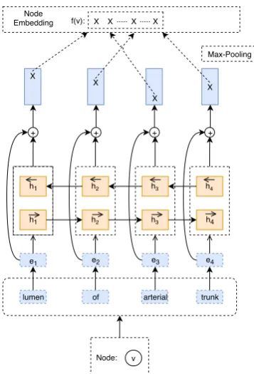
BIGRU-MAX-RES-N2V: This method uses a
bidirectional RNN (Schuster and Paliwal, 1997). For each node v with descriptor S(v) =
hw1, w2, . . . , wni, a bidirectional GRU (BIGRU)
computes two sets ofnhidden state vectors, one for each direction. These two sets are then added to form the outputHof theBIGRU:
Hf = GRUf(e(w1), . . . , e(wn)) (4)
Hb = GRUb(e(w1), . . . , e(wn)) (5)
H = Hf+Hb (6)
where f, b denote the forward and backward
di-rections, and + indicates component-wise addi-tion. We add residual connections (He et al.,2015) from each word embedding e(wt) to the
corre-sponding hidden state htofH. Instead of using
the final forward and backward states of H, we apply max-pooling (Collobert and Weston,2008;
Conneau et al.,2017) over the state vectors htof
H. The output of the max pooling is the node em-beddingf(v). Figure3illustrates this method.
Node: v
lumen of arterial trunk
e1 e2 e3 e4
h1
h1
h2
h2
h3
h3
h4
h4
+ + + +
X
X
X
X Node
Embedding f(v): X X ... X ... X
[image:5.595.89.268.68.331.2]Max-Pooling
Figure 3: Obtaining the embedding of a nodevby ap-plying aBIGRUencoder with max-pooling and residu-als to the embeddings ofv’s textual descriptor.
self-attention (Bahdanau et al., 2015) instead of max-pooling were also tried. To save space, we described only the best performing variant.
4 Experiments
We investigate the effectiveness of our proposed approach by conducting link prediction experi-ments on two biomedical datasets derived from UMLS. Furthermore, we devise a new approach of generating negative edges for the link predic-tion evaluapredic-tion – beyond just random negatives – that makes the problem more difficult and aligns more with real-world use-cases. We also conduct a qualitative analysis, showing that the proposed framework does indeed leverage both the textual descriptors and the network structure.
4.1 Datasets
We created our datasets from the UMLS ontol-ogy, which contains approx. 3.8 million biomed-ical concepts and 54 semantic relationships. The relationships become edges in the networks, and the concepts become nodes. Each concept (node) is associated with a textual descriptor. We extract two types of semantic relationships, creating two networks. The first, and smaller one, consists of PART-OFrelationships where each node represents a part of the human body. The second network
Statistics IS-A PART-OF
Nodes 294,693 16,894
Edges 356,541 19,436
Training true positive edges 294,692 16,893 Training true negative edges 294,692 16,893 Test true positive edges 61,849 2,543 Test true negative edges 61,849 2,543 Avg. descriptor length 5 words 6 words Max. descriptor length 31 words 14 words
Table 1: Statistics of the two datasets (IS-A,PART-OF). The true positive and true negative edges are used in the link prediction experiments.
containsIS-Arelationships, and the concepts rep-resented by the nodes vary across the spectrum of biomedical entities (diseases, proteins, genes, etc.). To our knowledge, theIS-Anetwork is one of the largest datasets employed for link predic-tion and learning network embeddings. Statistics for the two datasets are shown in Table1.
4.2 Baseline Node Embedding Methods
We compare our proposed methods to baselines of two types: structure-oriented methods, which solely focus on network structure, and content-oriented methods that try to combine the net-work structure with the textual descriptors of the nodes (albeit using impoverished network neigh-borhoods so far). For the first type of methods, we employ NODE2VEC (Grover and Leskovec,
2016), which uses a biased random walk algo-rithm based on DEEPWALK(Perozzi et al.,2014) to explore the structure of the network more ef-ficiently. Our work can be seen as an extension of NODE2VEC that incorporates textual node de-scriptors, as already discussed, hence it is natural to compare toNODE2VEC. As acontent-oriented
baseline we use CANE (Tu et al., 2017), which learns separate text-based and network-based em-beddings, and uses a mutual attention mechanism to dynamically change the text-based embeddings for different neighbors (Section 2). CANE only considers the direct neighbors of each node, un-likeNODE2VEC, which considers larger neighbor-hoods obtained via random walks.
4.3 Link Prediction
In link prediction, we are given a network with a certain fraction of edges removed. We need to infer these missing edges by observing the incom-plete network, facilitating the discovery of links (e.g., unobserved protein-protein interactions).
[image:5.595.309.518.71.164.2]the network remains connected so that we can per-form random walks over it. Each removed edgee connecting nodes v1, v2 is treated as a true pos-itive, in the sense that a link prediction method should infer that an edge should be added between v1, v2. We also use an equal number oftrue nega-tives, which are pairs of nodesv01, v02with no edge between v10, v20 in the original network. When evaluating NE methods, a link predictor is given true positive and true negative pairs of nodes, and is required to discriminate between the two classes by examining only the node embeddings of each pair. Node embeddings are obtained by applying aNE method to the pruned network, i.e., after re-moving the true positives. A NE method is con-sidered better than another one, if it leads to better performance of the same link predictor.
We experiment with two approaches to obtain true negatives. InRandom Negative Sampling, we randomly select pairs of nodes that were not di-rectly connected (by a single edge) in the original network. InClose Proximity Negative Sampling, we iterate over the nodes of the original network considering each one as a focus. For each focus nodev, we want to find another node u in close proximity that is not an ancestor or descendent (e.g., parent, grandparent, child, grandchild) ofv in the IS-A or PART-OF hierarchy, depending on the dataset. We wantuto be close tov, to make it more difficult for the link predictor to infer that u and v should not be linked. We do not, how-ever, want u to be an ancestor or descendent of v, because theIS-A andPART-OFrelationships of our datasets are transitive. For example, if u is a grandparent ofv, it could be argued that infer-ring thatu andv should be linked, is not an er-ror. To satisfy these constraints, we first find the ancestors ofv that are between 2 to 5 hops away fromvin the original network.3 We randomly se-lect one of these ancestors, and then we randomly select as u one of the ancestor’s children in the original network, ensuring that u was not an an-cestor or descendent ofvin the original network. In both approaches, we randomly select as many true negatives as the true positives, discarding the remaining true negatives.
We experimented with two link predictors:
Cosine similarity link predictor (CS): Given a
pair of nodesv1, v2(true positive or true negative
3
The edges of the resulting datasets are not directed. Hence, looking for descendents would be equivalent.
edge), CS computes the cosine similarity (ignor-ing negative scores) between the two node embed-dings as s(v1, v2) = max(0,cos(f(v1), f(v2))), and predicts an edge between the two nodes if s(v1, v2)≥t, wheretis a threshold. We evaluate the predictor on the true positives and true nega-tives (shown as ‘test’ true posinega-tives and ‘test’ true negatives in Table1) by computingAUC(area un-derROCcurve), in effect considering the precision and recall of the predictor for varyingt.4
Logistic regression link predictor (LR): Given a
pair of nodes v1, v2, LRcomputes the Hadamard (element-wise) product of the two node embed-dings f(v1)f(v2)and feeds it to a logistic re-gression classifier to obtain a probability estimate pthat the two nodes should be linked. The predic-tor predicts an edge betweenv1, v2 ifp ≥ t. We compute AUCon a test set by varyingt. The test set of this predictor is the same set of true pos-itives and true negatives (with Random or Close Proximity Negative Sampling) that we use when evaluating the CS predictor. The training set of the logistic regression classifier contains as true positives all the other edges of the network that remain after the true positives of the test set have been removed, and an equal number of true nega-tives (with the same negative sampling method as in the test set) that are not used in the test set.
4.4 Implementation Details
For NODE2VEC and our NE methods, which can be viewed as extensions of NODE2VEC, the di-mensionality of the node embeddings is 30. The dimensionality of the word embeddings (in ourNE methods) is also 30. In the random walks, we set r = 5, l = 40, k = 10 for IS-A, and r = 10, l = 40, k = 10 for PART-OF; these hyper-parameters were not particularly tuned, and their values were selected mostly to speed up the experiments. We train for one epoch with a batch size of 128, set-ting the number ofSKIPGRAM’s negative samples to 2. We use the Adam (Kingma and Ba,2015) op-timizer in ourNE methods. We implemented our NEmethods and the two link predictors using Py-Torch (Paszke et al.,2017) and Scikit-Learn (
Pe-dregosa et al.,2011). ForNODE2VECandCANE,
we used the implementations provided.5
4
We do not report precision, recall, F1 scores, because these require selecting a particular thresholdtvalues.
5
Random Close Negative Proximity NE Method + Link Predictor Sampling Sampling
Node2Vec + CS 66.6 54.3
CANE + CS 94.1 69.6
Avg-N2V + CS 95.0 78.6
GRU-N2V + CS 98.7 79.2
BiGRU-Max-Res-N2V + CS 98.5 79.0
Node2Vec + LR CANE + LR Avg-N2V + LR GRU-N2V + LR
BiGRU-Max-Res-N2V + LR
77.2 95.3 97.6 99.0
99.3
56.3 70.0 73.9 79.6
[image:7.595.77.288.72.218.2]82.1
Table 2: AUC scores (%) for the IS-A dataset. Best scores per link predictor (CS,LR) shown in bold.
For CANE, we set the dimensionality of the node embeddings to 200, as in the work ofTu et al.
(2017). We also tried 30-dimensional node em-beddings, as inNODE2VECand our NEmethods, but performance deteriorated significantly.
4.5 Link Prediction Results
Link prediction results for the IS-A and PART -OF networks are reported in Tables 2and3. All content-oriented NE methods (CANE and our ex-tensions of NODE2VEC) clearly outperform the structure-oriented method (NODE2VEC) on both datasets in both negative edge sampling settings, showing that modeling the textual descriptors of the nodes is critical. Furthermore, all methods perform much worse with Close Proximity Nega-tive Sampling, confirming that the latter produces more difficult link prediction datasets.
All of our NE methods (content-aware exten-sions ofNODE2VEC) outperformNODE2VECand CANE in every case, especially with Close Prox-imity Negative Sampling. We conclude that it is important to model not just the textual descriptor of a node or its direct neighbors, but as much non-local network structure as possible.
For PART-OFrelations (Table3),BIGRU-MAX -RES-N2V obtains the best results with both link predictors (CS,LR) in both negative sampling set-tings, but the differences fromGRU-N2Vare very small in most cases. For IS-A (Table 2), BIGRU -MAX-RES-N2V obtains the best results with the LR predictor, and only slightly inferior results thanGRU-N2Vwith the CSpredictor. The differ-ences of these twoNEmethods fromAVG-N2Vare larger, indicating that recurrent neural encoders of textual descriptors are more effective than simply averaging the word embeddings of the descriptors.
Random Close
Negative Proximity NE Method + Link Predictor Sampling Sampling
Node2Vec + CS 76.8 61.8
CANE + CS 93.9 75.3
Avg-N2V + CS 95.9 81.8
GRU-N2V + CS 98.0 83.1
BiGRU-Max-Res-N2V + CS 98.5 83.3
Node2Vec + LR CANE + LR Avg-N2V + LR GRU-N2V + LR
BiGRU-Max-Res-N2V + LR
85.2 94.4 97.6 99.0
99.5
66.5 76.3 79.4 85.6
[image:7.595.312.522.73.218.2]88.6
Table 3:AUCscores (%) for thePART-OFdataset. Best scores per link predictor (CS,LR) shown in bold.
Target Node:Left Eyeball (PART-OF)
Most Similar Embeddings Cos Hops
equator of left eyeball 99.3 1
episcleral layer of left eyeball 99.2 4
cavity of left eyeball 99.1 1
wall of left eyeball 99.0 1
vascular layer of left eyeball 98.9 1
Target Node:Lung Carcinoma (IS-A)
Most Similar Embeddings Cos Hops
recurrent lung
carcinoma 97.6 1
papillary carcinoma 97.1 2
lung pleomorphic
carcinoma 97.0 3
ureter carcinoma 96.6 2
lymphoepithelioma-like lung
carcinoma 96.6 3
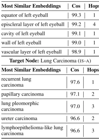
Table 4: Examples of nodes whose embeddings are closest (cosine similarity, Cos) to the embedding of a target node in thePART-OF(top) and IS-A(bottom) datasets. We also show the distances (number of edges, Hops) between the nodes in the networks.
[image:7.595.329.496.296.530.2](a) Two nodes connected by aPART-OFedge.
(b) Two nodes connected by aPART-OFedge.
[image:8.595.92.263.65.186.2](c) Two nodes connected by anIS-Aedge.
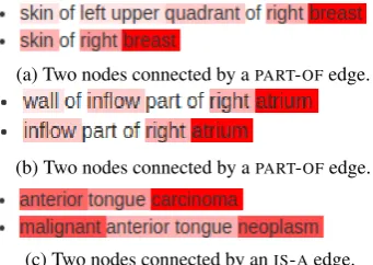
Figure 4: Visualization of the importance thatBIGRU
-MAX-RES-N2Vassigns to the words of the descriptors of the nodes of three edges. Edges (a) and (b) are from thePART-OFdataset. Edge (c) is from theIS-Adataset.
4.6 Qualitative Analysis
To better understand the benefits of leveraging both network structure and textual descriptors, we present examples from the two datasets.
Most similar embeddings: Table 4 presents the
five nearest nodes for two target nodes (‘Left Eye-ball’ and ‘Lung Carcinoma’), based on the cosine similarity of the corresponding node embeddings in the PART-OF and IS-A networks, respectively. We observe that all nodes in thePART-OFexample are very similar content-wise to our target node. Furthermore, the model captures the semantic lationship between concepts, since most of the re-turned nodes are actually parts of ‘Left Eyeball’. The same pattern is observed in theIS-Aexample, with the exception of ‘ureter carcinoma’, which is not directly related with ‘lung carcinoma’, but is still a form of cancer. Finally, it is clear that the model extracts meaningful information from both the textual content of each node and the network structure, since the returned nodes are closely lo-cated in the network (Hops 1–4).
Heatmap visualization: BIGRU-MAX-RES-N2V
can be extended to highlight the words in each textual descriptor that mostly influence the cor-responding node embedding. Recall that this NE method applies a max-pooling operator (Fig. 3) over the state vectors h1, . . . , hn of the words
w1, . . . , wn of the descriptor, keeping the
maxi-mum value per dimension across the state vectors. We count how many dimension-values the max-pooling operator keeps from each state vectorhi,
and we treat that count (normalized to [0,1]) as the importance score of the corresponding word wi.6 We then visualize the importance scores as
6
We actually obtain two importance scores for each word
Edges/Descriptors BN2V CANE N2V Hops
(a) bariatric surgery (b) bypass
gastrojejunostomy
82.7 38.0 56.2 11
(a) anatomical line (b) anterior malleolar fold
82.3 29.0 50.0 22
(a) zone of biceps brachii
(b) short head of biceps brachii
93.0 70.0 61.6 13
Table 5: Examples of true positive edges, showing how structure and textual descriptors affect node embed-dings. The first two edges are IS-A, the third one is
PART-OF. TheNEmethods used areBIGRU-MAX-RES
-N2V(BN2V),CANEandNODE2VEC(N2V). We report cosine similarities between node embeddings and the distances between the nodes (number of edges, Hops) in the networks after removing true positive edges.
heatmaps of the descriptors. In the first two exam-ple edges of Fig.4, the highest importance scores are assigned to words indicating body parts, which is appropriate given that the edges indicatePART -OFrelations. In the third example edge, the high-est importance score of the first descriptor is as-signed to ‘carcinoma’, and the highest importance scores of the second descriptor are shared by ‘ma-lignant’ and ‘neoplasm’; again, this is appropriate, since these words indicate anIS-Arelation.
Case Study: In Table5, we present examples that
illustrate learning from both the network struc-ture and textual descriptors. All three edges are true positives, i.e., they were initially present in the network and they were removed to test link prediction. In the first two edges, which come from theIS-Anetwork, the node descriptors share no words. Nevertheless, BIGRU-MAX-RES-N2V (BN2V) produces node embeddings with high co-sine similarities, much higher than NODE2VEC that uses only network structure, presumably be-cause the word embeddings (and neural encoder) of BN2V correctly capture lexical relations (e.g., near-synonyms). Although CANE also considers the textual descriptors, its similarity scores are much lower, presumably because it uses only local neighborhoods (single-edge hops). The nodes in the third example, which come from thePART-OF network, have a larger word overlap. NODE2VEC
[image:8.595.306.526.72.204.2]is unaware of this overlap and produces the lowest score. The two content-oriented methods (BN2V, CANE) produce higher scores, but again BN2V produces a much higher similarity, presumably because it uses larger neighborhoods. In all three edges, the two nodes are distant (>10 hops), yet BN2Vproduces high similarity scores.
5 Conclusions and Future Work
We proposed a new method to learn content-aware node embeddings, which extends NODE2VECby considering the textual descriptors of the nodes. The proposed approach leverages the strengths of both structure- and content-oriented node em-bedding methods. It exploits non-local network neighborhoods generated by random walks, as in the original NODE2VEC, and allows integrating various neural encoders of the textual descrip-tors. We evaluated our models on two biomed-ical networks extracted from UMLS, which con-sist of PART-OF and IS-A edges. Experimental results with two link predictors, cosine similar-ity and logistic regression, demonstrated that our approach is effective and outperforms previous methods which rely on structure alone, or model content along with local network context only.
In future work, we plan to experiment with net-works extracted from other biomedical ontologies and knowledge bases. We also plan to explore if the word embeddings that our methods generate can improve biomedical question answering sys-tems (McDonald et al.,2018).
Acknowledgements
This work was partly supported by the Research Center of the Athens University of Economics and Business. The work was also supported by the French National Research Agency under project ANR-16-CE33-0013.
References
Monica Agrawal, Marinka Zitnik, and Jure Leskovec. 2018. Large-scale analysis of disease pathways in the human interactome. Pacific Symposium on Biocomputing. Pacific Symposium on Biocomput-ing, 23:111–122.
Nesreen K. Ahmed, Ryan A. Rossi, John Boaz Lee, Xi-angnan Kong, Theodore L. Willke, Rong Zhou, and Hoda Eldardiry. 2018. Learning role-based graph embeddings. CoRR, abs/1802.02896.
Dzmitry Bahdanau, Kyunghyun Cho, and Yoshua Ben-gio. 2015. Neural machine translation by jointly learning to align and translate. In 3rd Inter-national Conference on Learning Representations, ICLR 2015, San Diego, CA, USA, May 7-9, 2015, Conference Track Proceedings.
James Bergstra, Daniel L K Yamins, and David D. Cox. 2013. Hyperopt: A python library for opti-mizing the hyperparameters of machine learning al-gorithms.
Olivier Bodenreider. 2004. The unified medical lan-guage system (UMLS): integrating biomedical ter-minology. Nucleic Acids Research, 32(Database-Issue):267–270.
Kyunghyun Cho, Bart van Merrienboer, C¸ aglar G¨ulc¸ehre, Dzmitry Bahdanau, Fethi Bougares, Hol-ger Schwenk, and Yoshua Bengio. 2014. Learning phrase representations using RNN encoder-decoder for statistical machine translation. InProceedings of the 2014 Conference on Empirical Methods in Nat-ural Language Processing, EMNLP 2014, October 25-29, 2014, Doha, Qatar, A meeting of SIGDAT, a Special Interest Group of the ACL, pages 1724– 1734.
Ronan Collobert and Jason Weston. 2008. A unified architecture for natural language processing: deep neural networks with multitask learning. In Ma-chine Learning, Proceedings of the Twenty-Fifth In-ternational Conference (ICML 2008), Helsinki, Fin-land, June 5-9, 2008, pages 160–167.
Alexis Conneau, Douwe Kiela, Holger Schwenk, Lo¨ıc Barrault, and Antoine Bordes. 2017. Supervised learning of universal sentence representations from natural language inference data. InProceedings of the 2017 Conference on Empirical Methods in Nat-ural Language Processing, EMNLP 2017, Copen-hagen, Denmark, September 9-11, 2017, pages 670– 680.
Aditya Grover and Jure Leskovec. 2016. node2vec: Scalable feature learning for networks. In KDD, pages 855–864. ACM.
Kaiming He, Xiangyu Zhang, Shaoqing Ren, and Jian Sun. 2015. Deep residual learning for image recog-nition.CoRR, abs/1512.03385.
Armand Joulin, Edouard Grave, Piotr Bojanowski, and Tomas Mikolov. 2016. Bag of tricks for efficient text classification.CoRR, abs/1607.01759.
Diederik P. Kingma and Jimmy Ba. 2015. Adam: A method for stochastic optimization. CoRR, abs/1412.6980.
Chengwei Lei and Jianhua Ruan. 2013. A novel link prediction algorithm for reconstructing protein-protein interaction networks by topological similar-ity.Bioinformatics, 29(3):355–364.
Linyuan Lu and Tao Zhou. 2010. Link predic-tion in complex networks: A survey. CoRR, abs/1010.0725.
Ryan McDonald, Georgios-Ioannis Brokos, and Ion Androutsopoulos. 2018. Deep relevance ranking us-ing enhanced document-query interactions. In Pro-ceedings of the Conference on Empirical Methods in Natural Language Processing, pages 1849–1860, Brussels, Belgium.
Tomas Mikolov, Ilya Sutskever, Kai Chen, Gregory S. Corrado, and Jeffrey Dean. 2013. Distributed repre-sentations of words and phrases and their composi-tionality. InNIPS, pages 3111–3119.
Pushkar Mishra, Marco Del Tredici, Helen Yan-nakoudakis, and Ekaterina Shutova. 2019. Abusive language detection with graph convolutional net-works. CoRR, abs/1904.04073.
Christopher J Mungall. 2004. Obol: Integrating lan-guage and meaning in bio-ontologies. Comparative and Functional Genomics, 5:509 – 520.
Philip V. Ogren, K. Bretonnel Cohen, George K. Acquaah-Mensah, Jens Eberlein, and Lawrence E Hunter. 2003. The compositional structure of gene ontology terms. Pacific Symposium on Biocom-puting. Pacific Symposium on Biocomputing, pages 214–25.
Philip V. Ogren, K. Bretonnel Cohen, and Lawrence E Hunter. 2004. Implications of compositionality in the gene ontology for its curation and usage.Pacific Symposium on Biocomputing. Pacific Symposium on Biocomputing, pages 174–85.
Adam Paszke, Sam Gross, Soumith Chintala, Gre-gory Chanan, Edward Yang, Zachary DeVito, Zem-ing Lin, Alban Desmaison, Luca Antiga, and Adam Lerer. 2017. Automatic differentiation in pytorch.
Fabian Pedregosa, Ga¨el Varoquaux, Alexandre Gram-fort, Vincent Michel, Bertrand Thirion, Olivier Grisel, Mathieu Blondel, Peter Prettenhofer, Ron Weiss, Vincent Dubourg, Jacob VanderPlas, Alexandre Passos, David Cournapeau, Matthieu Brucher, Matthieu Perrot, and Edouard Duch-esnay. 2011. Scikit-learn: Machine learning in python. Journal of Machine Learning Research, 12:2825–2830.
Bryan Perozzi, Rami Al-Rfou, and Steven Skiena. 2014. Deepwalk: online learning of social repre-sentations. InKDD, pages 701–710. ACM.
Michael Schlichtkrull, Thomas N Kipf, Peter Bloem, Rianne Van Den Berg, Ivan Titov, and Max Welling. 2018. Modeling relational data with graph convolu-tional networks. In European Semantic Web Con-ference, pages 593–607. Springer.
Mike Schuster and Kuldip K. Paliwal. 1997. Bidirec-tional recurrent neural networks. IEEE Trans. Sig-nal Processing, 45:2673–2681.
Prithviraj Sen, Galileo Namata, Mustafa Bilgic, Lise Getoor, Brian Gallagher, and Tina Eliassi-Rad. 2008. Collective classification in network data. AI Magazine, 29(3):93–106.
Dinghan Shen, Xinyuan Zhang, Ricardo Henao, and Lawrence Carin. 2018. Improved semantic-aware network embedding with fine-grained word align-ment. InProceedings of the 2018 Conference on Empirical Methods in Natural Language Process-ing, Brussels, Belgium, October 31 - November 4, 2018, pages 1829–1838.
Ali Shojaie. 2013. Link prediction in biological net-works using multi-mode exponential random graph models.
Xiaofei Sun, Jiang Guo, Xiao Ding, and Ting Liu. 2016. A general framework for content-enhanced network representation learning. CoRR, abs/1610.02906.
Jian Tang, Meng Qu, Mingzhe Wang, Ming Zhang, Jun Yan, and Qiaozhu Mei. 2015. LINE: large-scale in-formation network embedding. InProceedings of the 24th International Conference on World Wide Web, WWW 2015, Florence, Italy, May 18-22, 2015, pages 1067–1077.
Cunchao Tu, Han Liu, Zhiyuan Liu, and Maosong Sun. 2017. CANE: context-aware network embedding for relation modeling. InProceedings of the 55th Annual Meeting of the Association for Computa-tional Linguistics, ACL 2017, Vancouver, Canada, July 30 - August 4, Volume 1: Long Papers, pages 1722–1731.
Daixin Wang, Peng Cui, and Wenwu Zhu. 2016. Struc-tural deep network embedding. InProceedings of the 22nd ACM SIGKDD International Conference on Knowledge Discovery and Data Mining, San Francisco, CA, USA, August 13-17, 2016, pages 1225–1234.
Peng Wang, Baowen Xu, Yurong Wu, and Xiaoyu Zhou. 2015. Link prediction in social networks: the state-of-the-art.SCIENCE CHINA Information Sci-ences, 58(1):1–38.
Appendix
A CANE Hyper-parameters
CANE has 3 hyper-parameters, denoted α, β, γ, which control to what extent it uses information from network structure or textual descriptors. We learned these hyper-parameters by employing the HyperOpt (Bergstra et al., 2013) on the valida-tion set.7 All three hyper-parameters had the same search space:[0.2,1,0]with a step of0.1. The op-timization ran for 30 trials for both datasets. Ta-ble6reports the resulting hyper-parameter values.
Parameters PART-OF IS-A
α 0.2 0.7
β 1.0 0.7
γ 1.0 0.7
Table 6: Hyper-parameter values used inCANE.
7