Predicting CPI in Panama

(1)

Munich Personal RePEc Archive

Predicting CPI in Panama

NYONI, THABANI

UNIVERSITY OF ZIMBABWE

15 February 2019

Online at

https://mpra.ub.uni-muenchen.de/92419/

(2)

Predicting CPI in Panama

Nyoni, Thabani

Department of Economics

University of Zimbabwe

Harare, Zimbabwe

Email: [email protected]

ABSTRACT

This study uses annual time series data on CPI in Panama from 1960 to 2017, to model and forecast CPI using the Box – Jenkins ARIMA technique. Diagnostic tests indicate that the P series is I (1). The study presents the ARIMA (1, 1, 0) model for predicting CPI in Panama. The diagnostic tests further imply that the presented optimal model is actually stable and acceptable for forecasting CPI in Panama. The results of the study apparently show that CPI in Panama is likely to continue on an upwards trajectory in the next 10 years. The study encourages policy makers to make use of tight monetary and fiscal policy measures in order to deal with inflation in Panama.

Key Words: Forecasting, Inflation, Panama

JEL Codes: C53, E31, E37, E47

INTRODUCTION

(3)

reflector of inflationary trends in the economy, it is often treated as a litmus test of the effectiveness of economic policies of the government of the day (Sarangi et al, 2018). The CPI program focuses on consumer expenditures on goods and services out of disposable income (Boskin et al, 1998). Hence, it excludes non-market activity, broader quality of life issues, and the costs and benefits of most government programs (Kharimah et al, 2015). To avoid adjusting policy and models by not using an inflation rate prediction can result in imprecise investment and saving decisions, potentially leading to economic instability (Enke & Mehdiyev, 2014). Precisely forecasting the change of CPI is significant to many aspects of economics, some examples include fiscal policy, financial markets and productivity. Also, building a stable and accurate model to forecast the CPI will have great significance for the public, policy makers and research scholars (Du et al, 2014). In this study we use CPI as an indicator of inflation in Panama. The main objective of this endeavor is to model and forecast CPI in Panama using the Box-Jenkins ARIMA technique.

LITERATURE REVIEW

Zivko & Bosnjak (2017) investigated inflation in Croatia using ARIMA models with a data set ranging over the period January 1997 to November 2015 and discovered that the ARIMA (0, 1, 1)x(0, 1, 1)12 is the optimal model for forecasting inflation in Croatia. In Albania, Dhamo et al

investigated CPI using SARIMA models with a data set ranging over the period January 1994 to December 2007 and revealed that SARIMA models are satisfactory for a short-term prediction compared to the multiple regression model forecast. Nyoni (2018k) studied inflation in Zimbabwe using GARCH models with a data set ranging over the period July 2009 to July 2018 and established that there is evidence of volatility persistence for Zimbabwe’s monthly inflation data. Nyoni (2018n) modeled inflation in Kenya using ARIMA and GARCH models and relied on annual time series data over the period 1960 – 2017 and found out that the ARIMA (2, 2, 1) model, the ARIMA (1, 2, 0) model and the AR (1) – GARCH (1, 1) model are good models that can be used to forecast inflation in Kenya. Nyoni & Nathaniel (2019), based on ARMA, ARIMA and GARCH models; studied inflation in Nigeria using time series data on inflation rates from 1960 to 2016 and found out that the ARMA (1, 0, 2) model is the best model for forecasting inflation rates in Nigeria.

MATERIALS & METHODS

Box – Jenkins ARIMA Models

One of the methods that are commonly used for forecasting time series data is the Autoregressive Integrated Moving Average (ARIMA) (Box & Jenkins, 1976; Brocwell & Davis, 2002; Chatfield, 2004; Wei, 2006; Cryer & Chan, 2008). For the purpose of forecasting Consumer Price Index (CPI) in Panama, ARIMA models were specified and estimated. If the sequence

∆d

Pt satisfies an ARMA (p, q) process; then the sequence of Pt also satisfies the ARIMA (p, d, q)

process such that:

∆𝑑_𝑃

𝑡 = ∑ 𝛽𝑖∆𝑑𝑃𝑡−𝑖+ 𝑝

𝑖=1

∑ 𝛼𝑖𝜇𝑡−𝑖 𝑞

𝑖=1

+ 𝜇𝑡… … … . … … … … . … … . [1]

(4)

∆𝑑_𝑃

𝑡 = ∑ 𝛽𝑖∆𝑑𝐿𝑖𝑃𝑡 𝑝

𝑖=1

+ ∑ 𝛼𝑖𝐿𝑖𝜇𝑡 𝑞

𝑖=1

+ 𝜇𝑡… … … . . … … … . … … … [2]

where ∆ is the difference operator, vector β ϵⱤp and ɑ ϵⱤq.

The Box – Jenkins Methodology

The first step towards model selection is to difference the series in order to achieve stationarity. Once this process is over, the researcher will then examine the correlogram in order to decide on the appropriate orders of the AR and MA components. It is important to highlight the fact that this procedure (of choosing the AR and MA components) is biased towards the use of personal judgement because there are no clear – cut rules on how to decide on the appropriate AR and MA components. Therefore, experience plays a pivotal role in this regard. The next step is the estimation of the tentative model, after which diagnostic testing shall follow. Diagnostic checking is usually done by generating the set of residuals and testing whether they satisfy the characteristics of a white noise process. If not, there would be need for model re – specification and repetition of the same process; this time from the second stage. The process may go on and on until an appropriate model is identified (Nyoni, 2018i).

Data Collection

This study is based on a data set of annual CPI (P) in Panama ranging over the period 1960 – 2017. All the data was gathered from the World Bank.

Diagnostic Tests & Model Evaluation

Stationarity Tests

The ADF Test

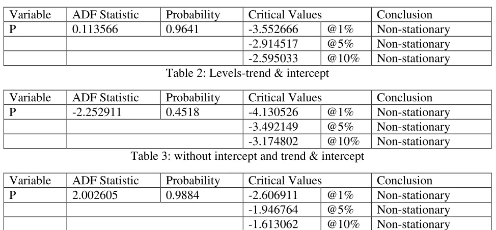
Table 1: Levels-intercept

Variable ADF Statistic Probability Critical Values Conclusion

P 0.113566 0.9641 -3.552666 @1% Non-stationary

[image:4.612.63.550.482.708.2]

-2.914517 @5% Non-stationary -2.595033 @10% Non-stationary Table 2: Levels-trend & intercept

P -2.252911 0.4518 -4.130526 @1% Non-stationary

-3.492149 @5% Non-stationary -3.174802 @10% Non-stationary Table 3: without intercept and trend & intercept

P 2.002605 0.9884 -2.606911 @1% Non-stationary

(5)

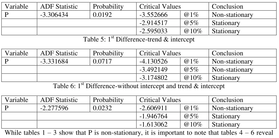
Table 4: 1st Difference-intercept

P -3.306434 0.0192 -3.552666 @1% Non-stationary

[image:5.612.64.550.92.333.2]

-2.914517 @5% Stationary -2.595033 @10% Stationary Table 5: 1st Difference-trend & intercept

P -3.331684 0.0717 -4.130526 @1% Non-stationary

-3.492149 @5% Non-stationary -3.174802 @10% Stationary Table 6: 1st Difference-without intercept and trend & intercept

P -2.277596 0.0232 -2.606911 @1% Non-stationary

-1.946764 @5% Stationary -1.613062 @10% Stationary

While tables 1 – 3 show that P is non-stationary, it is important to note that tables 4 – 6 reveal that P is an I (1) variable.

Evaluation of ARIMA models (with a constant)

Table 7

Model AIC U ME MAE RMSE MAPE

ARIMA (1, 1, 1) 204.4736 0.57927 0.016106 0.9356 1.3565 1.704

ARIMA (1, 1, 0) 202.5349 0.57853 0.018835 0.91764 1.3571 1.6711 ARIMA (0, 1, 1) 208.3152 0.64429 0.0047286 1.0477 1.4266 1.9421 ARIMA (2, 1, 1) 205.0353 0.58404 0.015878 0.95904 1.3392 1.7555 ARIMA (1, 1, 2) 204.6192 0.57722 0.024029 0.96391 1.3339 1.7418 ARIMA (2, 1, 2) 205.9163 0.57956 0.024755 0.95563 1.3255 1.7429 ARIMA (2, 1, 0) 204.5108 0.57874 0.017737 0.92448 1.3569 1.6838 A model with a lower AIC value is better than the one with a higher AIC value (Nyoni, 2018n). Theil’s U must lie between 0 and 1, of which the closer it is to 0, the better the forecast method (Nyoni, 2018l). The study will only consider the AIC as the criteria for choosing the best model for focasting CPI in Panama. The ARIMA (1, 1, 0) model was finally selected.

Residual & Stability Tests

ADF Tests of the Residuals of the ARIMA (1, 1, 0) Model

Table 8: Levels-intercept

Rt -7.223684 0.0000 -3.555023 @1% Stationary

(6)

Table 9: Levels-trend & intercept

Rt -7.194294 0.0000 -4.133838 @1% Stationary

-3.493692 @5% Stationary -3.175693 @10% Stationary Table 10: without intercept and trend & intercept

Rt -7.291151 0.0000 -2.607686 @1% Stationary

-1.946878 @5% Stationary -1.612999 @10% Stationary

Tables 8, 9 and 10 demonstrate that the residuals of the ARIMA (1, 1, 0) model are stationary and hence the ARIMA (1, 1, 0) is suitable for modeling CPI in Panama.

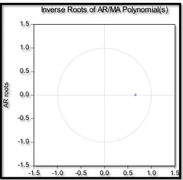
[image:6.612.172.439.319.581.2]

Stability Test of the ARIMA (1, 1, 0) Model

Figure 1

Since the corresponding inverse roots of the characteristic polynomial lie in the unit circle, it illustrates that the chosen ARIMA (1, 1, 0) model is indeed stable and suitable for predicting CPI in Panama over the period under study.

FINDINGS

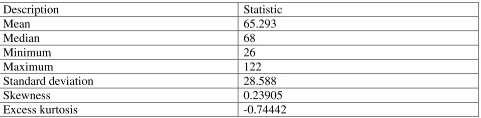
Descriptive Statistics

Table 11 -1.5

-1.0 -0.5 0.0 0.5 1.0 1.5

-1.5 -1.0 -0.5 0.0 0.5 1.0 1.5

A

R

r

o

ts

(7)

Description Statistic

Mean 65.293

Median 68

Minimum 26

Maximum 122

Standard deviation 28.588

Skewness 0.23905

Excess kurtosis -0.74442

As shown above, the mean is positive, i.e. 65.293. The minimum is 26 while the maximum is 122. The skewness is 0.23905 and the most striking characteristic is that it is positive, indicating that the P series is positively skewed and non-symmetric. Excess kurtosis is -0.74442; showing that the P series is not normally distributed.

Results Presentation1

Table 12

ARIMA (1, 1, 0) Model:

∆𝑃𝑡−1= 1.60596 + 0.668501∆𝑃𝑡−1… … … . … … … . … . [3]

P: (0.0051) (0.0000) S. E: (0.5051) (0.0979)

Variable Coefficient Standard Error z p-value

Constant 1.60596 0.505131 3.179 0.0051***

AR (1) 0.668501 0.0979399 6.826 0.0000***

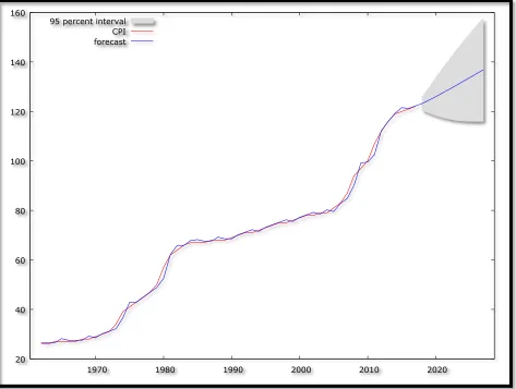
[image:7.612.69.548.70.188.2]

Forecast Graph

Figure 2

1

(8)

Predicted Annual CPI in Panama

Table 13

Year Prediction Std. Error 95% Confidence Interval

2018 123.20 1.350 120.56 - 125.85

2019 124.54 2.625 119.39 - 129.68

2020 125.96 3.879 118.36 - 133.56

2021 127.45 5.066 117.52 - 137.37

2022 128.97 6.173 116.87 - 141.07

2023 130.52 7.201 116.41 - 144.64

2024 132.09 8.156 116.11 - 148.08

2025 133.67 9.044 115.95 - 151.40

20 40 60 80 100 120 140 160

1970 1980 1990 2000 2010 2020

[image:8.612.79.552.76.433.2]

(9)

2026 135.26 9.874 115.91 - 154.62

2027 136.86 10.653 115.98 - 157.74

Figure 2 (with a forecast range from 2018 – 2027) and table 13, clearly show that CPI in Panama is indeed set to continue rising gradually, in the next 10 years.

POLICY IMPLICATION & CONCLUSION

After performing the Box-Jenkins approach, the ARIMA was engaged to investigate annual CPI of Panama from 1960 to 2017. The study mostly planned to forecast the annual CPI in Panama for the upcoming period from 2018 to 2027 and the best fitting model was selected based on how well the model captures the stochastic variation in the data. The ARIMA (1, 1, 0) model is not only stable but also the most suitable model to forecast the CPI of Panama for the next ten years. In general, CPI in Panama; showed an upwards trend over the forecasted period. Based on the results, policy makers in Panama should engage more proper economic and monetary policies in order to fight such increase in inflation as reflected in the forecasts. Therefore, monetary and fiscal authorities in Panama are encouraged to rely more on tight monetary policy, which should be accompanied by a tight fiscal policy stance.

REFERENCES

[1] Boskin, M. J., Ellen, R. D., Gordon, R. J., Grilliches, Z & Jorgenson, D. W (1998). Consumer Price Index and the Cost of Living, The Journal of Economic Perspectives, 12 (1): 3 – 26.

[2] Box, G. E. P & Jenkins, G. M (1976). Time Series Analysis: Forecasting and Control, Holden Day, San Francisco.

[3] Brocwell, P. J & Davis, R. A (2002). Introduction to Time Series and Forecasting, Springer, New York.

[4] Chatfield, C (2004). The Analysis of Time Series: An Introduction, 6th Edition, Chapman & Hall, New York.

[5] Cryer, J. D & Chan, K. S (2008). Time Series Analysis with Application in R, Springer, New York.

[6] Dhamo, E., Puka, L & Zacaj, O (2018). Forecasting Consumer Price Index (CPI) using time series models and multi-regression models (Albania Case Study), Financial Engineering, pp: 1 – 8.

[7] Du, Y., Cai, Y., Chen, M., Xu, W., Yuan, H & Li, T (2014). A novel divide-and-conquer model for CPI prediction using ARIMA, Gray Model and BPNN, Procedia Computer Science, 31 (2014): 842 – 851.

(10)

[9] Hurtado, C., Luis, J., Fregoso, C & Hector, J (2013). Forecasting Mexican Inflation Using Neural Networks, International Conference on Electronics, Communications and Computing, 2013: 32 – 35.

[10] Kharimah, F., Usman, M., Elfaki, W & Elfaki, F. A. M (2015). Time Series Modelling and Forecasting of the Consumer Price Bandar Lampung, Sci. Int (Lahore)., 27 (5): 4119 – 4624.

[11] Manga, G. S (1977). Mathematics and Statistics for Economics, Vikas Publishing House, New Delhi.

[12] Mcnelis, P. D & Mcadam, P (2004). Forecasting Inflation with Think Models and Neural Networks, Working Paper Series, European Central Bank.

[13] Nyoni, T & Nathaniel, S. P (2019). Modeling Rates of Inflation in Nigeria: An Application of ARMA, ARIMA and GARCH models, Munich University Library – Munich Personal RePEc Archive (MPRA), Paper No. 91351.

[14] Nyoni, T (2018k). Modeling and Forecasting Inflation in Zimbabwe: a Generalized Autoregressive Conditionally Heteroskedastic (GARCH) approach, Munich University Library – Munich Personal RePEc Archive (MPRA), Paper No. 88132.

[15] Nyoni, T (2018l). Modeling Forecasting Naira / USD Exchange Rate in Nigeria: a Box – Jenkins ARIMA approach, University of Munich Library – Munich Personal RePEc Archive (MPRA), Paper No. 88622.

[16] Nyoni, T (2018n). Modeling and Forecasting Inflation in Kenya: Recent Insights from ARIMA and GARCH analysis, Dimorian Review, 5 (6): 16 – 40.

[17] Nyoni, T. (2018i). Box – Jenkins ARIMA Approach to Predicting net FDI inflows in Zimbabwe, Munich University Library – Munich Personal RePEc Archive (MPRA), Paper No. 87737.

[18] Sarangi, P. K., Sinha, D., Sinha, S & Sharma, M (2018). Forecasting Consumer Price Index using Neural Networks models, Innovative Practices in Operations Management and Information Technology – Apeejay School of Management, pp: 84 – 93.

[19] Subhani, M. I & Panjwani, K (2009). Relationship between Consumer Price Index (CPI) and Government Bonds, South Asian Journal of Management Sciences, 3 (1): 11 – 17.

(11)