Fiscal Policy, Wages, and Jobs in the U S

Munich Personal RePEc Archive

Fiscal Policy, Wages, and Jobs in the

U.S.

Kim, Hyeongwoo

Auburn University

October 2018

Fiscal Policy, Wages, and Jobs in the U.S.

Hyeongwoo Kim

Auburn University

October 2018

Abstract

This paper empirically investigates the …scal policy e¤ects on labor market conditions, employing an array of structural vector autoregressive models for the post-war U.S. data from 1960:I to 2017:II. Fiscal spending shocks increase jobs in the government sector at the cost of private sector jobs, resulting in net losses to the total employment. Private wages increase insigni…cantly in the short-run, while government wages rise signi…cantly and persistently in response to the …scal shock. Consequently, the wage gap across the two sectors widens in response to the …scal shock. The wage shock yields signi…cantly positive responses of corporate pro…ts in the long-run as it enhances productivity, which supports wage-led growth models. On the other hand, I report negligible in-sample and out-of-in-sample predictive contents for private jobs and wages from corporate pro…ts, meaning that there’s virtually no evidence of the trickle-down e¤ect, which is essential for pro…t-led growth models.

Keywords: Government Spending; Labor Market Condition; Trickle-Down

Ef-fect; Pro…t-Led Growth; Wage-Led Growth; Out-of-Sample Forecast

JEL Classi…cation: E24; E52; E62

Special thanks go to Ehung Gi Baek, Kwanho Shin, Hangyu Lee, Hyeok Jeong, Shuwei Zhang, Randy Beard, and session participants at the 2017 KDI-JEP International Conference for helpful comments.

1

Introduction

The sluggish recovery from the recent Great Recession has revived the debate on the e¤ectiveness of the …scal policy in stimulating economic activity among the economics profession. Can increases in government spending help promote economic activity in the private sector? And if so, will key variables of interest such as consumption, in-vestment, employment, and real wages respond persistently positively to expansionary …scal policy? These questions has led to a large literature on this issue.

Some researchers are fairly optimistic about the role of government stimulus. They report overall positive responses of consumption, real wages, and output to expansion-ary government spending shocks, which are roughly in line with the New Keynesian macroeconomic model, even though replications of empirical …ndings can be di¢cult unless their models are heavily restricted. See, among others, Rotemberg and Wood-ford (1992), Devereux, Head, and Laphan (1996), Fatás and Mihov (2001), Blanchard and Perotti (2002), Perotti (2004), Galí, López-Salido, and Vallés (2007).

On the other hand, another group of scholars provides strong evidence of negative responses of consumption and real wages to …scal spending shocks. See, for example, Aiyagari, Christiano, and Eichenbaum (1992), Hall (1986), Ramey and Shapiro (1998), Edelberg, Eichenbaum, and Fisher (1999), Burnside, Eichenbaum, and Fisher (2004), Mountford and Uhlig (2009), Ramey (2012), and Owyang, Ramey, and Zubairy (2013). Ramey (2011b) points out that these responses re‡ect a negative wealth e¤ect that of-ten appears in the neoclassical macroeconomic model such as Aiyagari, Christiano, and Eichenbaum (1992) and Baxter and King (1993). Increases in government spending may result in a negative wealth e¤ect because the government has to raise tax in the future to …nance the de…cits. Rational consumers respond to it by reducing consump-tion and increase labor supply. Overall, empirical evidence on the e¤ectiveness of …scal stimulus is mixed.1

It should be noted that much of the attention in the literature has focused on the e¤ects of the …scal policy on the gross domestic product (GDP) and consumption,

whereas much less attention was paid to its e¤ects on labor market conditions, although policy-makers seems to have focused more on the latter in their e¤orts to combat the Great Recession.2

Some research works report a positive …scal policy e¤ect on employment as a by-product of its output e¤ects. See, among others, Fatás and Mihov (2001) and Burnside, Eichenbaum, and Fisher (2004). In contrast, some focused on its direct e¤ects on labor market variables. Finn (1998) demonstrates an increase in government jobs could result in a decrease in private sector employment. Cavallo (2005) proposes a similar model but with a dampened negative e¤ect on consumption as the government spending for public employment serves as a transfer for households. Monacelli, Perotti, and Trigari (2010) report more bene…cial e¤ects of the …scal policy on an array of labor market variables. Overall, the labor market e¤ects of …scal policy have been somewhat overlooked in the current literature, and we attempt to …ll the gap.

In this paper, we investigate the …scal policy e¤ects on labor market variables in the U.S. using an array of recursively identi…ed vector autoregressive (VAR) models, similar to the one by Blanchard and Perotti (2002), for the post-war macroeconomic data. Unlike Monacelli, Perotti, and Trigari (2010), we distinguish the key labor market variables in the private sector from those in the government sector. Unlike Finn (1998) and Cavallo (2005), we focus onempirical evidence of the …scal policy e¤ects on labor market conditions. Our major …ndings are as follows.

First, government spending shocks are not e¤ective in stimulating private activ-ity. The private gross domestic product that excludes government spending responds negatively to the …scal spending shock. Furthermore, its negative responses eventu-ally dominate increases in the government spending. Second, …scal spending shocks increase government jobs at the expense of private employment. Private and govern-ment wages both rise in response to expansionary …scal policy, although increases in private wages are overall insigni…cant. Government wages rise signi…cantly and per-sistently. Third, corporate pro…ts have virtually no role in improving the labor market conditions, meaning that there’s not much evidence of the so-called trickle-down e¤ect

that is crucial for pro…t-led economic growth models. Also, increases in productivity have limited e¤ects in enhancing labor market conditions.

Lastly, we corroborate these in-sample evidence with an array of out-of-sample fore-casting exercises that statistically evaluate predictive contents of key macroeconomic variables for wages and employment in the future. Government spending seems to have substantial and signi…cant out-of-sample predictive contents for employment. Private GDP contains some useful information for dynamics of wages and jobs in the future. On the contrary, corporate pro…ts have virtually no predictive contents for jobs and wages, which is again at odds with implications of the trickle-down e¤ect. Again, pro-ductivity provides limited information for out-of-sample prediction of private jobs and wages.

The remainder of this paper is organized as follows. Section 2 introduces our VAR models and out-of-sample forecast schemes. In Section 3, we present data descriptions and our major empirical …ndings. We also report an array of robustness check ana-lyses and simulation exercises. Section 4 reports our out-of-sample forecasting exercise results. Section 5 concludes.

2

The Econometric Model

We employ the following vector autoregressive (VAR) model.

x_t= 0d_t+

p X

j=1

A_jx_{t j+}Cu_{t; (1)}

where

x_{t = [gt yt labt it mt]}0_;

d_{t is a vector of deterministic terms that includes an intercept and time trend,} C _{is a}

lower-triangular matrix, andu_{t is a vector of mutually orthonormal structural shocks,}

that is, Eu_tu0

t = I. gt denotes the real federal government consumption and gross

investment spending per capita,yt is the real GDP per capita,labt is the labor market

variable,it is the e¤ective federal funds rate, and mt denotes the monetary base.

We are particularly interested in thej-period ahead orthogonalized impulse-response functions (OIRF) de…ned as follows.

where uk;t is the structural shock to the kth variable in (1) and t 1 is the adaptive

information set at time t 1.3

We also consider the private real GDP per capita (pgdpt) foryt in (1), which does

not include the total government consumption and gross investment. For labt, we

employ one of the following four labor market condition variables: private sector wages (pwt), government sector wages (gwt), private sector employment (pjt), and government

sector employment (gjt).

Note that gt is ordered …rst in (1), meaning that gt is not contemporaneously

in‡uenced by innovations in other variables within one quarter. This assumption is often employed in the current literature (e.g., Blanchard and Perotti [2002] and Ramey [2011a]), because implementations of discretionary …scal policy actions normally require Congressional approvals, which take longer than one quarter. On the other hand, the money market variables,itand mt, are ordered last. This is because the Federal Open

Market Committee (FOMC) can revise the stance of monetary policy via regular and emergency meetings whenever it is necessary. it is ordered beforemt because the Fed

targets the interest rate and the monetary base responds endogenously.

It is well documented that econometric inferences from recursively identi…ed VAR models may not be robust to alternative VAR ordering. However, Christiano, Eichen-baum, and Evans (1999) show that impulse-response functions can be invariant when the location of the shocking variable is …xed. It turns out that all response functions to the …scal spending shocks are numericallyidentical even when one randomly rearranges the variables next togt.4 Therefore, our key …ndings presented in this paper are robust

to alternative ordering.

In addition to the VAR model (1) for in-sample analysis, we employ the following autoregressive (AR) typeout-of-sample forecasting model to study the predictive con-tents for labor market variables in other macroeconomic variableszt. For this purpose,

we use the following j-period ahead AR(1)-type prediction model. Abstracting from deterministic terms, the benchmark forecasting model is,

labt+j = jlabt+ut+j; j = 1;2; ::; k; (3)

where j is less than one in absolute value for stationarity. Note that we employ a

3_{That is, the information set has the following property,}

t 1 t 2 t 3 .

direct forecasting approach by regressing labt+j on the current value labt. It should

be also noted that j coincides with the AR(1) persistence parameter ( 1 = ) when

j = 1.5 _{The ordinary least squares (OLS) estimator for (3) yields the followingj-period}

ahead forecast from this benchmark AR-type model.

labBMt+jjt= ^jlabt (4)

We propose the following competing model that extends (3) with a predictor vari-able zt.

labt+j = jlabt+ jzt+ut+j; j = 1;2; ::; k (5)

Applying the OLS estimator for (5), we obtain the following j-period ahead forecast for the target variable from this competing model,

labC_t+jjt= ^jlabt+ ^jzt (6)

Note that the competing model (5) nests the stationary benchmark model (3) whenzt

does not contain any useful predictive contents forlabt+j, that is, j = 0.

We implement out-of-sample forecast exercises, employing a …xed-size rolling win-dow method that performs better than recursive methods in the presence of a structural break.

We …rst estimate the coe¢cients in our forecasting models (3) and (5) using the initialT0 < T observations,flabt; ztgT

0

t=1, then obtain thej period ahead out-of-sample

forecast for the target variable,labT0+j by (4) or (6). Next, we move the sample period

of the data forward by adding one more observation to the sample but dropping one earliest observation,flabt; ztg

T0+1

t=2 , then re-estimate the coe¢cients for the next round

forecast for labT0+j+1. Note that we maintain the same number of observations (T0)

throughout the whole exercises. We repeat until we forecast the last observation,

labT. We implement this scheme for up to 12 quarter (3 years) forecast horizons,

j = 1;2; :::;12.

For evaluations of the out-of-sample prediction accuracy, we use the ratio of the

5_{Forj >1,}

root mean square prediction error (RRMSPE) de…ned as follows,

RRM SP E(j) =

r

1

T T0 j

PT

t=T0+j u

BM t+jjt

2

r

1

T T0 j

PT

t=T0+j u

C t+jjt

2; (7)

where

uBM_t+jjt =labt+j labBMt+jjt; u C

t+jjt=labt+j labCt+jjt (8)

Note that our competing model outperforms the benchmark model whenRRMSPE is greater than1.

We supplement our analyses by employing the Diebold-Mariano-West (DMW) test. See Diebold and Mariano (1995) and West (1996). For this, we de…ne the following loss function,

dt= (uBMt+jjt)

2

(uC t+jjt)

2

; (9)

where the squared loss function can be replaced by the absolute value loss function. The DMW statistic is de…ned as follows to test the null of equal predictive accuracy, that is,H0 :Edt= 0,

DM W(j) = q d

[

Avar(d)

; (10)

wheredis the sample average,d= 1

T T0 j

PT

t=T0+jdt, andAvar(d)[ denotes the

asymp-totic variance ofd,

[

Avar(d) = 1 T T0

q X

i= q

k(i; q)^i;

where k( ) is a kernel function with the bandwidth parameter q, and ^i is the ith

autocovariance function estimate.

3

Empirical Findings

3.1

Data Descriptions

We obtained all data from the Federal Reserve Economic Data (FRED). Observations are quarterly frequency and span from 1960:I to 2017:II.

The private GDP (pyt) is the total GDP (yt) minus the total government

consump-tion and gross investment spending (tgt). That is, tgt include the federal government

spending (gt) as well as those of the state and local governments. All income/spending

variables are log-transformed and are expressed in real per capita terms using the GDP de‡ator and total population. The money market variables are the e¤ective fed-eral funds rate (EFFR,it) and the monetary base (MB,mt), which are used to control

the e¤ect of monetary policy.

The private wage (pwt) is the total compensation in the private sector (A132RC1Q027SBEA)

divided by the GDP de‡ator and the number of employees in the total private industries (USPRIV;pjt). The government sector wage (gwt) denotes the total compensation in

the government sector (B202RC1Q027SBEA) divided by the GDP de‡ator and the number of employees in the government (USGOVT; gjt). In addition to the private

sector jobs (pjt) and the government sector jobs (gjt), we also use the total nonfarm

employment (PAYEMS;tjt) in our baseline VAR models.

The corporate pro…ts (prft) is the nominal corporate pro…ts after tax (CP) divided

by the GDP de‡ator, which is log-transformed. We consider the following two measures of productivity (prdt): real output per person in nonfarm business sector (OPHNFB)

and real output per hour of all persons in nonfarm business sector (PRS85006163). Both are log-transformed and yielded similar results, so we report …ndings with the second measure of productivity.

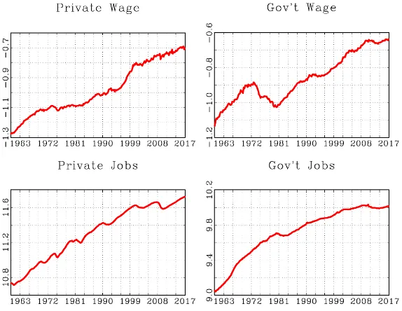
Figure 1 reports time series graphs of key macroeconomic data in panel (a) and of labor market variables in panel (b). All variables exhibit an upward trend over time. In order to check the business cycle properties of the data, we apply the Hodrick-Prescott (HP) …lter to the data with a smoothing parameter of 1,600 for quarterly data. Figure 2 reports the cyclical components along with the NBER recession dates marked in shaded areas.

By construction, the real GDP per capita (yt) tends to decrease (increase) when

the economy enters a downturn (boom) phase. The federal government spending (gt)

im-plemented by the federal government. The corporate pro…ts and the real hourly output (productivity) tend to show procyclical dynamics. Private wages and jobs overall ex-hibit comovements and are procyclical, while government wages and jobs often increase during economic downturns. It should be noted that the wage gap (gwt pwt) and the

job ratio (gjt pjt) show strong counter-cyclical movements. That is, the wage gap

and the job ratio tends to rise rapidly during economic downturns. In what follows, we show that these changes can be explained by expansionary government spending shocks.

Figures 1 and 2 around here

3.2

VAR Analysis

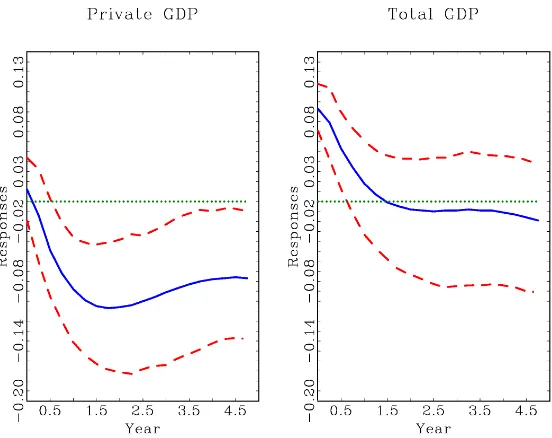
This subsection reports an array of the impulse-response function estimates based on (1) and (2) along with the one standard deviation con…dence bands that are generated from 500 nonparametric bootstrap simulations. We …rst report responses of the real GDP variables (yt and pyt) to the …scal spending shock (gt) in Figure 3 based on

x_{t = [gt pyt tjt it mt]}0 _and x_{t = [gt yt tjt it mt]}0_{, where tjt is the total nonfarm}

employment.

One notable …nding is that the government spending (gt) shock is ine¤ective in

stimulating private activity (pyt). The initial increase in the real GDP (yt) is driven

mainly by the increase in the government spending because the private spending barely responds to the shock in the short-run. Eventually, the real GDP responses become negligible as the private GDP declines, cancelling out the increase in the government spending.6

Figure 3 around here

In Figure 4, we report …scal policy e¤ects on key labor market variables. As can be seen in the upper panel (a), the government spending shock has a statistically

6_{The monetary policy shock, identi…ed by a negative ( ) 1% shock to the EFFR (i}

signi…cant positive e¤ect only on the government sector wages (gwt). Its e¤ect on the

private sector wages (pwt) is statistically insigni…cant, although its point estimates stay

positive for about 2 years. The wage gap (gwt pwt) responds positively, meaning that

public sector workers are more likely to bene…t from …scal policy shocks.

It turns out that these responses are closely related with those of employment in the private and the government sectors that are reported in the lower panel (b). In response to the government spending shock, private jobs (pjt) declines signi…cantly for

about 4 years, while government sector jobs (gjt) increase signi…cantly for over a year.

It should be noted that these responses are likely to occur when the government implements value-added type policy instead of government purchases. That is, when the government hires more workers, private sector labor may move to the government sector, which results in a decrease in the labor supply in the private sector. Strong demand in the government labor market raises the government wages, while a decrease in the labor supply in the private sector also increases the private wages.7

Figures 4 around here

We noticed that the …scal policy has not been quite successful in improving the labor market condition. We next investigate how other economic variables in‡uence the labor market condition. The …rst variable we consider is the after-tax corporate pro…t (prft), motivated by the so-called trickle-down e¤ect that often appear in

pro…t-led growth models. These models claim that labor market condition would improve when businesses prosper because the strong demand for labor generates more jobs and higher wages.

In response to the 1% corporate pro…t shock, private wages respond signi…cantly positively for about a year. See Figure 5. However, its responses are quantitatively weak and short-lived, which implies a very limited support for the trickle-down e¤ect in the U.S.8

It should be noted, however, that the corporate pro…t (prft) rises signi…cantly

in the long-run in response to a 1% private wage shock, although it initially decreases

7_{Monetary policy tends to strengthen labor market conditions in both sectors. Expansionary} monetary policy stimulates private spending that creates the stronger labor demand in the private sector. As the economy grows, the demand for public services also grows, then labor market conditions in the public sector improve endogenously.

re‡ecting higher manufacturing costs. One explanation may be found from statistically signi…cant positive responses of the productivity (prdt) to a private wage shock. See

Figure 6. That is, higher wages in the private sector may improve working environment, thus increase labor productivity, then contributes to higher corporate pro…ts in the long-run. Note that these responses are consistent with the e¢ciency wage hypothesis.9

Private wages respond signi…cantly positively for less than 2 years when the pro-ductivity shock occurs, implying that workers garner a limited amount of bene…ts of higher productivity.

Figures 5 and 6 around here

3.3

Robustness Check

This sub-section reports an array of robustness check analysis. We …rst investigate the stability of our key VAR …ndings over time. Among others, we are particularly interested in …scal policy e¤ects on labor market variables in Figure 4.

For this, I employ a 30-year rolling window scheme to repeatedly estimate the impulse-response functions over di¤erent sample periods. I start with estimations of the impulse-response functions using the …rst 30-year long data. Then, I moved the sample period forward by adding one new observation but dropping one oldest observation, which is used to obtain the second set of the impulse-response functions. I repeat until I estimate the response functions using the last 30-year long data.

Graphs in Figure 7 show fairly consistent sets of the impulse-response function estimates. In response to the …scal spending shock, private jobs (pjt) decrease then

recover in two or more years. Total employment (tjt) exhibits similar responses,

mean-ing that increases in government jobs (gjt) are dominated by decreases in private jobs.

Private wages (pwt) rise a little, whereas government wages (gwt) rise more

substan-tially.

Figure 7 around here

Next, we implement the forecast error variance decomposition (FEVDEC) analysis for private sector wages and jobs. The purpose of this exercise is to measure the further in-sample evidence of the trickle-down e¤ect. When the business condition improves and corporate pro…ts rise, workers may be able to share the gains eventually. In panel (a) of Figure 8, I report the share of corporate pro…t shock in explaining the total variation of private wages or jobs in up to 5 years. In addition to the corporate pro…t shock, I also added the real GDP shock as another explanatory variable, and the remaining explanatory power is assumed to be due to the private wage shock as residuals.

Surprisingly, corporate pro…ts have virtually no explanatory power for future private wages in all forecast horizons we consider. On the other hand, the share of the real GDP continuously rise up to almost 50% in 5 years. Similarly, corporate pro…ts have negligible explanatory power for private jobs in all forecast horizons.

In panel (b), we implement a similar FEVDEC analysis to measure the role of pro-ductivity in explaining private labor market conditions. It turns out that propro-ductivity has virtually no explanatory power for future private wages in all forecast horizons. However, it has some (15 to 20%) explanatory power for private jobs.

These …ndings again imply very limited evidence of the trickle-down e¤ect. Private wages fail to bene…t from increases in corporate pro…ts. Higher productivity seems to generate jobs in the private sector but fails to generate higher wages. In addition to these in-sample evidence, we further investigate the validity of the trickle-down e¤ect employing the out-of-sample forecasting framework in Section 4.

Figure 8 around here

3.4

Simulation Exercises

Private jobs fall signi…cantly below the deterministic time trend line when the …scal spending shock occurs. The job losses reach over 12 millions of jobs in about 3 years in annual rate as can be seen in Table 1. Government jobs signi…cantly increase above the trend line only for a short period of time, and eventually are dominated by decreases in private jobs.

Private wages rise for about 2 and a half year, then declines below the trend. Overall, the responses of private wages are statistically insigni…cant. On the other hand, government wages increase highly signi…cantly for over 5 years. Increases in government wages are substantial and overall dominate the decreases in private wages in longer term, widening the wage gap between the two sectors.

Figures 9 and 10 around here

Table 1 around here

4

Out-of-Sample Forecast Exercises

This section investigates what variables contain predictive contents for our key labor market variables under the out-of-sample forecasting framework described earlier in Section 2. For this purpose, we employ the model (5) that augments an AR(1) type benchmark prediction model (3) of the labor market variable (labt) with an extra

predictor of interest (zt) to see whether zt provides additional predictive power to the

benchmark model.

We consider the following four labor market variables for labt: private jobs (pjt),

government jobs (gjt), private wages (pwt), and government wages (gwt). For the

predictor variable (zt), we use the government spending (gt), corporate pro…ts (prft),

productivity (prdt), and the private GDP (pyt). We report the RRMSPE and the DMW statistics for each exercise in Tables 2 and 3.

As can be seen in Table 2,gtcontains strong out-of-sample predictive contents forpjt

1 year. These out-of-sample …ndings corroborate our earlier in-sample evidence that …scal policy tends to strengthen the public job market at the expense of private jobs.

Other variables add a lot weaker performance in our out-of-sample forecast exer-cises. prft and pyt have additional predictive contents only in a few cases. That is,

I fail to …nd out-of-sample evidence in favor of the trickle-down e¤ect, which corrob-orates my previous in-sample evidence. prdt seems to have stronger performance in

the medium-run than prft and pyt for pjt. Interestingly, pyt seems to have

substan-tial predictive contents forgjt, which implies that the demand for government services

increases as the economy ‡ourishes.

Table 2 around here

Table 3 reports theRRMSPE andDMW statistics for wage variables,pwtand gwt.

gt and prft add virtually no additional predictive contents for private wages (pwt),

which again implies virtually no evidence of the trickle-down e¤ect. prdt and pyt have

some predictive contents for it in the long-run and in the short-run, respectively. For government sector wages (gwt), I …nd very limited or virtually no predictive contents

from all variables we consider. gtdoes not have much out-of-sample predictive contents

for gwt, although it does an important role in explaining gwt in previous in-sample

analysis. In a nutshell, these predictor variables play very weak roles in forecasting wage dynamics in the near future.

Table 3 around here

5

Conclusion

Corporate pro…ts have negligible e¤ects on private wages, which provides strong empirical evidence against the trickle-down e¤ect. Increases in productivity have sig-ni…cantly positive e¤ect on private wages only in the short-run. On the other hand, positive wage shocks in the private sector increase corporate pro…ts in the long-run, re‡ecting signi…cant productivity improvement in response to the wage shock. Our robustness check analysis via the FEVDEC and sub-sample analysis overall con…rms these …ndings. We also implement simulation exercises to numerically assess how wages and jobs evolve over time in response to the …scal spending shock in comparison with the dynamic path with no structural shocks. Results imply that the …scal shock shrinks private sector employment substantially, while government wages rise signi…cantly and substantially, widening the wage gap between the two sectors.

References

Aiyagari, S. R., L. J. Christiano, and M. Eichenbaum (1992): “The output,

employment, and interest rate e¤ects of government consumption,”Journal of Mon-etary Economics, 30(1), 73–86.

Auerbach, A. J., and Y. Gorodnichenko (2012): “Fiscal multipliers in recession

and expansion,” in Fiscal Policy after the Financial Crisis, NBER Chapters, pp. 63–98. National Bureau of Economic Research, Inc.

Bachmann, R., and E. R. Sims (2012): “Con…dence and the transmission of

gov-ernment spending shocks,” Journal of Monetary Economics, 59(3), 235–249.

Baxter, M.,and R. G. King (1993): “Fiscal policy in general equilibrium,”

Amer-ican Economic Review, 83(3), 315–34.

Blanchard, O., and R. Perotti (2002): “An empirical characterization of the

dynamic e¤ects of changes in government spending and taxes on output,” The Quarterly Journal of Economics, 107(4), 1329–1368.

Burnside, C., M. Eichenbaum, and J. D. M. Fisher (2004): “Fiscal shocks and

their consequences,” Journal of Economic Theory, 115(1), 89–117.

Cavallo, M.(2005): “Government Employment Expenditure and the E¤ects of Fiscal

Policy Shocks,” Working Paper Series 2005-16, Federal Reserve Bank of San Fran-cisco.

Christiano, L., M. Eichenbaum, and S. Rebelo (2011): “When Is the

Govern-ment Spending Multiplier Large?,”Journal of Political Economy, 119(1), 78–121.

Christiano, L. J., M. Eichenbaum, and C. L. Evans (1999): “Monetary policy

shocks: What have we learned and to what end?,” in Handbook of Macroeconomics, ed. by J. B. Taylor, and M. Woodford, Handbook of Macroeconomics, chap. 2, pp. 65–148. Elsevier.

Devereux, M. B., A. C. Head,andB. J. Lapham (1996): “Monopolistic

Diebold, F. X., and R. S. Mariano (1995): “Comparing Predictive Accuracy,”

Journal of Business & Economic Statistics, 13(3), 253–263.

Edelberg, W., M. Eichenbaum, and J. D. Fisher (1999): “Understanding the

e¤ects of a shock to government purchases,” Review of Economic Dynamics, 2(1), 166–206.

Fatás, A., and I. Mihov (2001): “The e¤ects of …scal policy on consumption and

employment: Theory and evidence,” CEPR Discussion Papers 2760, C.E.P.R.

Fazzari, S. M., J. Morley, and I. Panovska (2015): “State-dependent e¤ects of

…scal policy,” Studies in Nonlinear Dynamics & Econometrics, 19(3), 285–315.

Finn, M. G.(1998): “Cyclical E¤ects of Government’s Employment and Goods

Pur-chases,” International Economic Review, 39(3), 635–57.

Galí, J., J. D. López-Salido, and J. Vallés (2007): “Understanding the e¤ects

of government spending on consumption,” Journal of the European Economic Asso-ciation, 5(1), 227–270.

Hall, R. E. (1986): “The role of consumption in economic ‡uctuations,” in The

American Business Cycle: Continuity and Change, NBER Chapters, pp. 237–266. National Bureau of Economic Research, Inc.

Kim, H.,andB. Jia(2017): “Government Spending Shocks and Private Activity: The

Role of Sentiments,” Auburn Economics Working Paper 2017-08, Auburn University.

McCracken, M. W. (2007): “Asymptotics for out of sample tests of Granger

caus-ality,”Journal of Econometrics, 140(2), 719–752.

Mittnik, S.,and W. Semmler(2012): “Regime dependence of the …scal multiplier,”

Journal of Economic Behavior and Organization, 83, 502–522.

Monacelli, T., R. Perotti, and A. Trigari (2010): “Unemployment …scal

mul-tipliers,”Journal of Monetary Economics, 57(5), 531–553.

Mountford, A., and H. Uhlig (2009): “What are the e¤ects of …scal policy

Owyang, M. T., V. A. Ramey,and S. Zubairy(2013): “Are government spending multipliers greater during periods of slack? Evidence from 20th century historical data,” NBER Working Papers 18769, National Bureau of Economic Research, Inc.

Perotti, R. (2004): “Estimating the e¤ects of …scal policy in OECD countries,”

Working Papers 276, IGIER (Innocenzo Gasparini Institute for Economic Research), Bocconi University.

Ramey, V. A.(2011a): “Can government purchases stimulate the economy?,”Journal

of Economic Literature, 49:3, 673–685.

(2011b): “Identifying government spending shocks: It’s all in the timing,”

The Quarterly Journal of Economics, 126(1), 1–50.

(2012): “Government spending and private activity,” in Fiscal Policy after the Financial Crisis. NBER conference.

Ramey, V. A., and M. D. Shapiro (1998): “Costly capital reallocation and the

e¤ects of government spending,” Carnegie-Rochester Conference Series on Public Policy, 48(1), 145–194.

Ramey, V. A., and S. Zubairy (2014): “Government spending multipliers in good

times and in bad: Evidence from U.S. historical data,” NBER Working Papers 20719, National Bureau of Economic Research, Inc.

Rotemberg, J. J.,andM. Woodford(1992): “Oligopolistic pricing and the e¤ects

of aggregate demand on economic activity,” Journal of Political Economy, 100(6), 1153–1207.

West, K. D.(1996): “Asymptotic Inference about Predictive Ability,”Econometrica,

Figure 1. The Data

(a) Macroeconmic Data

(b) Labor Market Data

Figure 2. Business Cycle Components of the Data

(a) Macroeconmic Data

(b) Labor Market Data

Figure 3. Fiscal Policy Effects on the Real Gross Domestic Product

Note: Prior to estimations, all variables were demeaned and detrended with up to a quadratic time trend. The first panel reports response function estimates to a 1% posi-tive shock to the government consumption and gross investment (gt). Dashed lines are

Figure 4. Fiscal Policy Effects on Labor Market Conditions

(a) Wage Effects

(b) Employment Effects

Note: We estimate the impulse-response function with the total GDP.The wage gap is defined as the log government sector wage minus the log private sector wage. The job ratio is the log government sector employment minus the private sector employment. Prior to estimations, all variables were demeaned and detrended with up to a quadratic time trend. We report response function estimates to a 1% positive shock to the government consumption and gross investment (gt). Dashed lines are 1 standard deviation confidence

Figure 5. Corporate Profits and Wages

Note: We estimate the impulse-response function based onx′t= [gt, yt, pwt, prft, it, mt]

′

. Prior to estimations, all variables were demeaned and detrended with up to a quadratic time trend. The first figure is the response function estimates of the private wages (pwt)

to a 1% positive shock to the corporate profits after tax (prft). The second figure is the

response of the corporate profits after tax (prft)to a 1% positive shock to the real wage

in the private sector (pwt). Dashed lines are 1 standard deviation confidence intervals

Figure 6. Productivity and Real Wages

Note: We estimate the impulse-response function based onx′t= [gt, yt, prdt, pwt, it, mt]

′

. Prior to estimations, all variables were demeaned and detrended with up to a quadratic time trend. The first figure is the response function estimates of the private wages (pwt)

to a 1% positive shock to the productivitiy (prdt). The second figure is the response

of the productivity (prdt)to a 1% positive shock to the real wage in the private

sec-tor (pwt).Dashed lines are 1 standard deviation confidence intervals obtained from 500

Figure 7. 30-Year Fixed Rolling Window Analysis

(a) Government Spending Shock Effects on Jobs

(b) Government Spending Shock Effects on Wages

Figure 8. Forecast Error Variance Decomposition Analysis

(a) Share of Corporate Profits

(b) Share of Productivity

Note: We estimate the forecast error variance decomposition for the labor variable in the private sector, that is, x′t= [yt, pwt, prft]

′

, [yt, pjt, prft]

′

, [yt, prdt, pwt]

′

, and

[yt, prdt, pjt]

′

Figure 9. Simulation Exercises: Employment Effects

(a) Private Jobs

(b) Government Jobs

Figure 10. Simulation Exercises: Wage Effects

(a) Private Wages

(b) Government Wages

Table 1. Gains or Losses to the 1% Fiscal Spending Shock

j (year) pjobt gjobt pwagt gwagt

0.25 1,257 1,013 401 4,020 0.50 −2,371 951 1,987 2,950

0.75 −5,466 959 1,267 3,910

1.00 −7,933 967 1,166 4,600

1.50 −11,064 959 708 5,830

2.00 −12,433 951 253 6,670

3.00 −11,325 855 −554 7,600

4.00 −8,810 699 −1,358 7,560

5.00 −7,166 452 −2,110 6,860

Table 2. h-Period ahead Out-of-Sample Forecast for Employment

(a) Private Jobs

Gov’t Spending Profits Productivity Private GDP

h RRMSPE DMW RRMSPE DMW RRMSPE DMW RRMSPE DMW

1 1.021 3.463 1.017 1.358 0.977 −2.435 1.006 0.283

2 1.016 2.235 1.005 0.542 0.978 −2.750 1.000 0.019

3 1.012 1.421 0.996 −0.743 0.982 −2.623 0.997 −0.220

4 1.009 0.998 0.989 −2.505 0.987 −2.421 0.996 −0.404

5 1.006 0.648 0.986 −4.002 0.992 −1.910 0.996 −0.470

6 1.005 0.561 0.983 −3.751 0.997 −0.794 0.997 −0.462

7 1.006 0.694 0.984 −3.193 1.003 1.397 0.998 −0.439

8 1.008 0.932 0.986 −2.335 1.008 4.051 0.999 −0.181

9 1.008 0.896 0.991 −1.290 1.013 5.059 1.001 0.475

10 1.011 1.215 0.999 −0.165 1.018 5.222 1.004 2.261

11 1.017 1.913 1.009 0.930 1.025 4.960 1.010 3.417

12 1.024 2.388 1.021 1.980 1.034 4.887 1.020 3.685

(b) Government Jobs

Gov’t Spending Profits Productivity Private GDP

h RRMSPE DMW RRMSPE DMW RRMSPE DMW RRMSPE DMW

1 1.014 1.098 0.994 −0.614 0.962 −1.322 1.039 0.708

2 1.022 1.500 0.986 −1.128 0.923 −2.297 1.087 1.283

3 1.021 1.514 0.979 −1.749 0.889 −3.838 1.127 1.580

4 1.009 0.723 0.976 −2.604 0.866 −4.401 1.186 2.633

5 0.991 −0.635 0.974 −3.260 0.864 −4.042 1.230 3.249

6 0.963 −2.183 0.971 −3.826 0.877 −3.748 1.301 4.514

7 0.931 −3.481 0.968 −3.609 0.892 −3.431 1.368 6.859

8 0.896 −4.783 0.958 −3.553 0.913 −2.689 1.413 8.779

9 0.866 −6.929 0.939 −3.805 0.943 −1.742 1.413 9.463

10 0.837 −6.272 0.913 −4.420 0.979 −0.594 1.401 9.875

11 0.816 −8.834 0.890 −5.195 1.008 0.245 1.359 10.008

12 0.799 −7.530 0.864 −6.707 1.027 0.766 1.309 9.637

Table 3. h-Period ahead Out-of-Sample Forecast for Wages

(a) Private Wages

Gov’t Spending Profits Productivity Private GDP

h RRMSPE DMW RRMSPE DMW RRMSPE DMW RRMSPE DMW

1 0.995 −0.420 1.002 0.313 0.996 −0.888 1.017 0.649

2 0.988 −0.624 0.994 −0.890 0.975 −3.669 1.022 0.802

3 0.981 −0.958 0.986 −1.904 0.963 −4.744 1.018 0.677

4 0.979 −1.052 0.972 −3.627 0.955 −4.208 1.016 0.794

5 0.977 −1.195 0.963 −4.515 0.957 −5.146 1.008 0.330

6 0.974 −1.271 0.958 −6.254 0.963 −3.631 1.001 0.056

7 0.972 −1.693 0.953 −7.000 0.975 −2.054 0.991 −0.514

8 0.973 −1.280 0.953 −6.971 0.983 −1.336 0.999 −0.060

9 0.970 −1.704 0.946 −8.676 0.999 −0.176 0.995 −0.269

10 0.966 −1.914 0.942 −8.250 1.007 1.393 0.998 −0.125

11 0.972 −1.731 0.937 −9.623 1.011 2.256 1.005 0.284

12 0.978 −1.398 0.932 −8.265 1.012 2.324 1.010 0.535

(b) Government Wages

Gov’t Spending Profits Productivity Private GDP

h RRMSPE DMW RRMSPE DMW RRMSPE DMW RRMSPE DMW

1 0.918 −2.740 0.980 −0.511 0.973 −1.557 0.976 −1.719

2 0.831 −5.697 0.959 −0.917 0.948 −2.539 0.949 −3.323

3 0.784 −6.163 0.940 −1.302 0.922 −2.798 0.927 −3.484

4 0.739 −9.372 0.920 −2.202 0.901 −4.434 0.907 −5.848

5 0.732 −11.041 0.922 −2.238 0.890 −5.094 0.913 −5.237

6 0.713 −11.737 0.915 −2.618 0.878 −5.762 0.929 −4.721

7 0.702 −13.716 0.908 −3.241 0.860 −6.660 0.953 −2.764

8 0.688 −17.030 0.893 −4.417 0.850 −8.659 0.990 −0.633

9 0.679 −17.354 0.889 −5.107 0.843 −8.300 1.048 3.048

10 0.662 −17.919 0.881 −5.456 0.839 −8.998 1.116 6.753

11 0.642 −19.761 0.866 −6.853 0.829 −9.504 1.183 9.348

12 0.620 −21.858 0.854 −7.411 0.829 −10.960 1.267 13.411