Proceedings of the 55th Annual Meeting of the Association for Computational Linguistics, pages 123–135 Vancouver, Canada, July 30 - August 4, 2017. c2017 Association for Computational Linguistics Proceedings of the 55th Annual Meeting of the Association for Computational Linguistics, pages 123–135
Vancouver, Canada, July 30 - August 4, 2017. c2017 Association for Computational Linguistics
A Convolutional Encoder Model for Neural Machine Translation
Jonas Gehring, Michael Auli, David Grangier, Yann N. Dauphin
Facebook AI Research
Abstract
The prevalent approach to neural machine translation relies on bi-directional LSTMs to encode the source sentence. We present a faster and simpler architecture based on a succession of convolutional layers. This al-lows to encode the source sentence simulta-neously compared to recurrent networks for which computation is constrained by tem-poral dependencies. On WMT’16 English-Romanian translation we achieve compet-itive accuracy to the state-of-the-art and on WMT’15 English-German we outper-form several recently published results. Our models obtain almost the same accuracy as a very deep LSTM setup on WMT’14 English-French translation. We speed up CPU decoding by more than two times at the same or higher accuracy as a strong
bi-directional LSTM.1
1 Introduction
Neural machine translation (NMT) is an end-to-end
approach to machine translation (Sutskever et al.,
2014). The most successful approach to date
en-codes the source sentence with a bi-directional re-current neural network (RNN) into a variable length representation and then generates the translation left-to-right with another RNN where both com-ponents interface via a soft-attention mechanism (Bahdanau et al.,2015;Luong et al.,2015a; Brad-bury and Socher, 2016; Sennrich et al., 2016a). Recurrent networks are typically parameterized as long short term memory networks (LSTM; Hochre-iter et al. 1997) or gated recurrent units (GRU; Cho et al. 2014), often with residual or skip
connec-tions (Wu et al.,2016;Zhou et al.,2016) to enable
stacking of several layers (§2).
There have been several attempts to use convo-lutional encoder models for neural machine trans-1The source code will be availabe athttps://github.
com/facebookresearch/fairseq
lation in the past but they were either only ap-plied to rescoring n-best lists of classical systems (Kalchbrenner and Blunsom, 2013) or were not
competitive to recurrent alternatives (Cho et al.,
2014a). This is despite several attractive properties of convolutional networks. For example, convolu-tional networks operate over a fixed-size window of the input sequence which enables the simultaneous computation of all features for a source sentence. This contrasts to RNNs which maintain a hidden state of the entire past that prevents parallel com-putation within a sequence.
A succession of convolutional layers provides a shorter path to capture relationships between
ele-ments of a sequence compared to RNNs.2 This also
eases learning because the resulting tree-structure applies a fixed number of non-linearities compared to a recurrent neural network for which the number of non-linearities vary depending on the time-step. Because processing is bottom-up, all words un-dergo the same number of transformations, whereas for RNNs the first word is over-processed and the last word is transformed only once.
In this paper we show that an architecture based on convolutional layers is very competitive to recur-rent encoders. We investigate simple average pool-ing as well as parameterized convolutions as an al-ternative to recurrent encoders and enable very deep convolutional encoders by using residual
connec-tions (He et al., 2015;§3).
We experiment on several standard datasets and compare our approach to variants of recurrent en-coders such as uni-directional and bi-directional LSTMs. On WMT’16 English-Romanian transla-tion we achieve accuracy that is very competitive to the current state-of-the-art result. We perform competitively on WMT’15 English-German, and nearly match the performance of the best WMT’14 English-French system based on a deep LSTM setup when comparing on a commonly used subset 2For kernel width k and sequence length n we require
max1,ln−1 k−1
m
forwards on a succession of stacked convo-lutional layers compared tonforwards with an RNN.
of the training data (Zhou et al. 2016;§4,§5).
2 Recurrent Neural Machine Translation
The general architecture of the models in this work follows the encoder-decoder approach with soft
at-tention first introduced in (Bahdanau et al.,2015).
A source sentencex= (x1, . . . , xm)ofmwords is
processed by an encoder which outputs a sequence of statesz= (z1. . . . , zm).
The decoder is an RNN network that computes a
new hidden state si+1 based on the previous state
si, an embedding gi of the previous target
lan-guage wordyi, as well as a conditional inputci
de-rived from the encoder output z. We use LSTMs
(Hochreiter and Schmidhuber,1997) for all decoder
networks whose statesi comprises of a cell vector
and a hidden vectorhiwhich is output by the LSTM
at each time step. We input ci into the LSTM by
concatenating it togi.
The translation model computes a distribution
over the V possible target words yi+1 by
trans-forming the LSTM outputhivia a linear layer with
weightsWoand biasbo:
p(yi+1|y1, . . . , yi,x) = softmax(Wohi+1+bo)
The conditional input ci at time i is computed
via a simple dot-product style attention
mecha-nism (Luong et al.,2015a). Specifically, we
trans-form the decoder hidden state hi by a linear layer
with weights Wd and bd to match the size of the
embedding of the previous target wordgi and then
sum the two representations to yield di.
Condi-tional inputciis a weighted sum of attention scores
ai ∈ Rm and encoder outputs z. The attention
scoresai are determined by a dot product between
hi with each zj, followed by a softmax over the
source sequence:
di=Wdhi+bd+gi,
aij =
exp dT
i zj
Pm
t=1exp dTi zt
, ci= m
X
j=1 aijzj
In preliminary experiments, we did not find the
MLP attention of (Bahdanau et al.,2015) to perform
significantly better in terms of BLEU nor perplex-ity. However, we found the dot-product attention to be more favorable in terms of training and evalua-tion speed.
We use bi-directional LSTMs to implement
re-current encoders similar to (Zhou et al., 2016)
which achieved some of the best WMT14 English-French results reported to date. First, each word
of the input sequence x is embedded in
distribu-tional space resulting ine= (e1, . . . , em). The
em-beddings are input to two stacks of uni-directional RNNs where the output of each layer is reversed before being fed into the next layer. The first stack takes the original sequence while the second takes the reversed input sequence; the output of the sec-ond stack is reversed so that the final outputs of the stacks align. Finally, the top-level hidden states of the two stacks are concatenated and fed into a linear
layer to yieldz. We denote this encoder architecture
as BiLSTM.
3 Non-recurrent Encoders
3.1 Pooling Encoder
A simple baseline for non-recurrent encoders is the
pooling model described in (Ranzato et al., 2015)
which simply averages the embeddings of k
con-secutive words. Averaging word embeddings does not convey positional information besides that the words in the input are somewhat close to each other. As a remedy, we add position embeddings to encode the absolute position of each source word within a sentence. Each source embedding
ej therefore contains a position embedding lj as
well as the word embedding wj. Position
embed-dings have also been found helpful in memory net-works for question-answering and language
model-ing (Sukhbaatar et al.,2015). Similar to the
recur-rent encoder (§2), the attention scoresaij are
com-puted from the pooled representationszj, however,
the conditional input ci is a weighted sum of the
embeddingsej, notzj, i.e.,
ej =wj+lj, zj = 1
k
bXk/2c
t=−bk/2c
ej+t,
ci = m
X
j=1 aijej
The input sequence is padded prior to pooling such that the encoder output matches the input length
|z|=|x|. We setkto5in all experiments as (
Ran-zato et al.,2015).
3.2 Convolutional Encoder
A straightforward extension of pooling is to learn the kernel in a convolutional neural network (CNN).
The encoder outputzj contains information about a
fixed-sized context depending on the kernel width
be addressed by stacking several layers of convolu-tions followed by non-linearities: additional layers increase the total context size while non-linearities can modulate the effective size of the context as
needed. For instance, stacking5convolutions with
kernel width k = 3 results in an input field of11
words, i.e., each output depends on11input words,
and the non-linearities allow the encoder to exploit the full input field, or to concentrate on fewer words as needed.
To ease learning for deep encoders, we add resid-ual connections from the input of each convolution to the output and then apply the non-linear
activa-tion funcactiva-tion to the output (tanh; He et al., 2015);
the non-linearities are therefore not ’bypassed’. Multi-layer CNNs are constructed by stacking sev-eral blocks on top of each other. The CNNs do not contain pooling layers which are commonly used for down-sampling, i.e., the full source sequence length will be retained after the network has been applied. Similar to the pooling model, the convolu-tional encoder uses position embeddings.
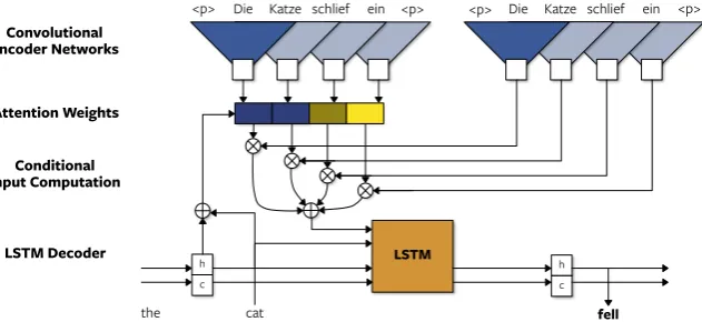
The final encoder consists of two stacked
convo-lutional networks (Figure1): CNN-aproduces the
encoder output zj to compute the attention scores
ai, while the conditional inputci to the decoder is
computed by summing the outputs ofCNN-c,
zj = CNN-a(e)j, ci =
m
X
j=1
aijCNN-c(e)j.
In practice, we found that two different CNNs re-sulted in better perplexity as well as BLEU
com-pared to using a single one (§5.3). We also found
this to perform better than directly summing the ei
without transformation as for the pooling model.
3.3 Related Work
There are several past attempts to use convolutional encoders for neural machine translation, however, to our knowledge none of them were able to match
the performance of recurrent encoders. (
Kalch-brenner and Blunsom, 2013) introduce a convolu-tional sentence encoder in which a multi-layer CNN generates a fixed sized embedding for a source sentence, or an n-gram representation followed by transposed convolutions for directly generating a per-token decoder input. The latter requires the length of the translation prior to generation and both models were evaluated by rescoring the output of
an existing translation system. (Cho et al.,2014a)
propose a gated recursive CNN which is repeat-edly applied until a fixed-size representation is
ob-tained but the recurrent encoder achieves higher ac-curacy. In follow-up work, the authors improved the model via a soft-attention mechanism but did not
re-consider convolutional encoder models (Bahdanau
et al.,2015).
Concurrently to our work, (Kalchbrenner et al.,
2016) have introduced convolutional translation
models without an explicit attention mechanism but their approach does not yet result in
state-of-the-art accuracy. (Lamb and Xie, 2016) also
pro-posed a multi-layer CNN to generate a fixed-size encoder representation but their work lacks
quan-titative evaluation in terms of BLEU. Meng et al.
(2015) and (Tu et al.,2015) applied convolutional
models to score pairs of traditional phrase-based and dependency-phrase-based translation models. Convolutional architectures have also been success-ful in language modeling but so far failed to
outper-form LSTMs (Pham et al.,2016).
4 Experimental Setup
4.1 Datasets
We evaluate different encoders and ablate architec-tural choices on a small dataset from the German-English machine translation track of IWSLT
2014 (Cettolo et al., 2014) with a similar setting
to (Ranzato et al.,2015). Unless otherwise stated, we restrict training sentences to have no more than 175 words; test sentences are not filtered. This is a higher threshold compared to other publications but ensures proper training of the position embed-dings for non-recurrent encoders; the length thresh-old did not significantly effect recurrent encoders. Length filtering results in 167K sentence pairs and
we test on the concatenation of tst2010, tst2011,
tst2012, tst2013anddev2010comprising 6948
sen-tence pairs.3 Our final results are on three major
WMT tasks:
WMT’16 English-Romanian. We use the same
data and pre-processing as (Sennrich et al.,2016a)
and train on 2.8M sentence pairs.4 Our model is
word-based instead of relying on byte-pair
encod-ing (Sennrich et al., 2016b). We evaluate on
new-stest2016.
WMT’15 English-German. We use all available
parallel training data, namely Europarl v7, Com-3Different to the other datasets, we lowercase the training
data and evaluate with case-insensitive BLEU.
4We followed the pre-processing of https:
h
h LSTM
Die Katze schlief ein <p>
<p> <p> Die Katze schlief ein <p>
the cat fell
c c
Convolutional Encoder Networks
Attention Weights
Conditional Input Computation
[image:4.595.135.451.58.203.2]LSTM Decoder
Figure 1: Neural machine translation model with single-layer convolutional encoder networks. CNN-ais
on the left andCNN-cis at the right. Embedding layers are not shown.
mon Crawl and News Commentary v10 and ap-ply the standard Moses tokenization to obtain 3.9M
sentence pairs (Koehn et al., 2007). We report
re-sults onnewstest2015.
WMT’14 English-French. We use a commonly
used subset of 12M sentence pairs (Schwenk,
2014), and remove sentences longer than 150
words. This results in 10.7M sentence-pairs for
training. Results are reported onntst14.
A small subset of the training data serves as vali-dation set (5% for IWSLT’14 and 1% for WMT) for
early stopping and learning rate annealing (§4.3).
For IWSLT’14, we replace words that occur fewer
than 3 times with a<unk>symbol, which results in
a vocabulary of 24158 English and 35882 German word types. For WMT datasets, we retain 200K source and 80K target words. For English-French only, we set the target vocabulary to 30K types to be comparable with previous work.
4.2 Model parameters
We use 512 hidden units for both recurrent encoders and decoders. We reset the decoder hidden states to zero between sentences. For the convolutional en-coder, 512 hidden units are used for each layer in
CNN-a, while layers in CNN-c contain 256 units
each. All embeddings, including the output pro-duced by the decoder before the final linear layer, are of 256 dimensions. On the WMT corpora, we find that we can improve the performance of the bi-directional LSTM models (BiLSTM) by using 512-dimensional word embeddings.
Model weights are initialized from a uniform
distribution within [−0.05,0.05]. For
convolu-tional layers, we use a uniform distribution of
−kd−0.5, kd−0.5, wherekis the kernel width (we
use 3 throughout this work) anddis the input size
for the first layer and the number of hidden units
for subsequent layers (Collobert et al.,2011b). For
CNN-c, we transform the input and output with
a linear layer each to match the smaller embed-ding size. The model parameters were tuned on IWSLT’14 and cross-validated on the larger WMT corpora.
4.3 Optimization
Recurrent models are trained with Adam as we found them to benefit from aggressive optimization.
We use a step width of3.125·10−4 and early
stop-ping based on validation perplexity (Kingma and
Ba, 2014). For non-recurrent encoders, we obtain
best results with stochastic gradient descent (SGD) and annealing: we use a learning rate of 0.1 and once the validation perplexity stops improving, we reduce the learning rate by an order of magnitude
each epoch until it falls below10−4.
For all models, we use mini-batches of 32 sen-tences for IWSLT’14 and 64 for WMT. We use truncated back-propagation through time to limit the length of target sequences per mini-batch to 25 words. Gradients are normalized by the mini-batch size. We re-normalize the gradients if their norm
exceeds 25 (Pascanu et al.,2013). Gradients of
con-volutional layers are scaled bysqrt(dim(input))−1
similar to (Collobert et al.,2011b). We use dropout
on the embeddings and decoder outputshi with a
rate of 0.2 for IWSLT’14 and 0.1 for WMT (
Sri-vastava et al.,2014). All models are implemented
in Torch (Collobert et al.,2011a) and trained on a
single GPU.
4.4 Evaluation
ran-dom seeds (5 for IWSLT’14, 3 for WMT) and pick the one with the best validation perplex-ity for final BLEU evaluation. Translations are generated by a beam search and we normalize
log-likelihood scores by sentence length. On
IWSLT’14 we use a beam width of 10 and for WMT models we tune beam width and word
penalty on a separate test set, that is newsdev2016
for WMT’16 English-Romanian, newstest2014
for WMT’15 English-German and ntst1213 for
WMT’14 English-French.5 The word penalty adds
a constant factor to log-likelihoods, except for the end-of-sentence token.
Prior to scoring the generated translations against the respective references, we perform unknown
word replacement based on attention scores (Jean
et al.,2015). Unknown words are replaced by look-ing up the source word with the maximum atten-tion score in a pre-computed dicatten-tionary. If the dictionary contains no translation, then we simply copy the source word. Dictionaries were extracted from the aligned training data that was aligned with
fast align (Dyer et al., 2013). Each source word is mapped to the target word it is most fre-quently aligned to.
For convolutional encoders with stackedCNN-c
layers we noticed for some models that the atten-tion maxima were consistently shifted by one word. We determine this per-model offset on the above-mentioned development sets and correct for it. Fi-nally, we compute case-sensitive tokenized BLEU, except for WMT’16 English-Romanian where we usedetokenizedBLEU to be comparable with Sen-nrich et al.(2016a).6
5 Results
5.1 Recurrent vs. Non-recurrent Encoders
We first compare recurrent and non-recurrent en-coders in terms of perplexity and BLEU on IWSLT’14 with and without position embeddings
(§3.1) and include a phrase-based system (Koehn
et al.,2007). Table1shows that a single-layer con-volutional model with position embeddings (Con-volutional) can outperform both a uni-directional LSTM encoder (LSTM) as well as a bi-directional LSTM encoder (BiLSTM). Next, we increase the depth of the convolutional encoder. We choose a 5Specifically, we select a beam from{5,10}and a word
penalty from{0,−0.5,−1,−1.5}
6https://github.com/moses-smt/
mosesdecoder/blob/617e8c8ed1630fb1d1/ scripts/generic/{multi-bleu.perl, mteval-v13a.pl}
System/Encoder BLEU BLEU PPL wrd+pos wrd wrd+pos
Phrase-based – 28.4 –
LSTM 27.4 27.3 10.8
BiLSTM 29.7 29.8 9.9
Pooling 26.1 19.7 11.0
Convolutional 29.9 20.1 9.1
Deep Convolutional 6/3 30.4 25.2 8.9
Table 1: Accuracy of encoders with position fea-tures (wrd+pos) and without (wrd) in terms of BLEU and perplexity (PPL) on IWSLT’14 Ger-man to English translation; results include unknown word replacement. Deep Convolutional 6/3 is the only multi-layer configuration, more layers for the LSTMs did not improve accuracy on this dataset.
good setting by independently varying the number
of layers inCNN-aandCNN-cbetween 1 and 10
and obtained best validation set perplexity with six
layers forCNN-aand three layers forCNN-c. This
configuration outperforms BiLSTM by 0.7 BLEU (Deep Convolutional 6/3). We investigate depth in
the convolutional encoder more in§5.3.
Among recurrent encoders, the BiLSTM is 2.3 BLEU better than the uni-directional version. The simple pooling encoder which does not contain any parameters is only 1.3 BLEU lower than a uni-directional LSTM encoder and 3.6 BLEU lower than BiLSTM. The results without position em-beddings (words) show that position information is crucial for convolutional encoders. In particu-lar for shallow models (Pooling and Convolutional), whereas deeper models are less effected. Recurrent encoders do not benefit from explicit position in-formation because this inin-formation can be naturally extracted through the sequential computation.
When tuning model settings, we generally ob-serve good correlation between perplexity and BLEU. However, for convolutional encoders per-plexity gains translate to smaller BLEU
improve-ments compared to recurrent counterparts (Table1).
We observe a similar trend on larger datasets.
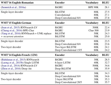
5.2 Evaluation on WMT Corpora
Next, we evaluate the BiLSTM encoder and the convolutional encoder architecture on three larger tasks and compare against previously published re-sults. On WMT’16 English-Romanian translation
we compare to (Sennrich et al., 2016a), the
WMT’16 English-Romanian Encoder Vocabulary BLEU
(Sennrich et al.,2016a) BiGRU BPE 90K 28.1
Single-layer decoder BiLSTM 80K 27.5
Convolutional 80K 27.1
Deep Convolutional 8/4 80K 27.8
WMT’15 English-German Encoder Vocabulary BLEU
(Jean et al.,2015) RNNsearch-LV BiGRU 500K 22.4 (Chung et al.,2016) BPE-Char BiGRU Char 500 23.9 (Yang et al.,2016) RNNSearch + UNK replace BiLSTM 50K 24.3
+ recurrent attention BiLSTM 50K 25.0
Single-layer decoder BiLSTM 80K 23.5
Deep Convolutional 8/4 80K 23.6
Two-layer decoder Two-layer BiLSTM 80K 24.1
Deep Convolutional 15/5 80K 24.2
WMT’14 English-French (12M) Encoder Vocabulary BLEU
(Bahdanau et al.,2015) RNNsearch BiGRU 30K 28.5 (Luong et al.,2015b) Single LSTM 6-layer LSTM 40K 32.7 (Jean et al.,2014) RNNsearch-LV BiGRU 500K 34.6 (Zhou et al.,2016) Deep-Att Deep BiLSTM 30K 35.9
Single-layer decoder BiLSTM 30K 34.3
Deep Convolutional 8/4 30K 34.6
Two-layer decoder 2-layer BiLSTM 30K 35.3
[image:6.595.114.486.59.342.2]Deep Convolutional 20/5 30K 35.7
Table 2: Accuracy on three WMT tasks, including results published in previous work. For deep
convolu-tional encoders, we include the number of layers inCNN-aandCNN-c, respectively.
They use byte pair encoding (BPE) to achieve open-vocabulary translation and dropout in all compo-nents of the neural network to achieve 28.1 BLEU;
we use the same pre-processing but no BPE (§4).
The results (Table 2) show that a deep
convo-lutional encoder can perform competitively to the
state of the art on this dataset (Sennrich et al.,
2016a). Our bi-directional LSTM encoder baseline is 0.6 BLEU lower than the state of the art but uses only 512 hidden units compared to 1024. A single-layer convolutional encoder with embedding size 256 performs at 27.1 BLEU. Increasing the
num-ber of convolutional layers to 8 in CNN-a and 4
inCNN-cachieves 27.8 BLEU which outperforms
our baseline and is competitive to the state of the art.
On WMT’15 English to German, we compare to
a BiLSTM baseline and prior work: (Jean et al.,
2015) introduce a large output vocabulary; the
decoder of (Chung et al., 2016) operates on the
character-level; (Yang et al.,2016) uses LSTMs
in-stead of GRUs and feeds the conditional input to the output layer as well as to the decoder.
Our single-layer BiLSTM baseline is competi-tive to prior work and a two-layer BiLSTM encoder performs 0.6 BLEU better at 24.1 BLEU.
Previ-ous work also used multi-layer setups, e.g., (Chung
et al., 2016) has two layers both in the encoder
and the decoder with 1024 hidden units, and (Yang
et al.,2016) use 1000 hidden units per LSTM. We use 512 hidden units for both LSTM and convolu-tional encoders. Our convoluconvolu-tional model with
ei-ther 8 or 15 layers inCNN-aoutperform the
BiL-STM encoder with both a single decoder layer or two decoder layers.
Finally, we evaluate on the larger WMT’14 English-French corpus. On this dataset the recur-rent architectures benefit from an additional layer both in the encoder and the decoder. For a single-layer decoder, a deep convolutional encoder outper-forms the BiLSTM accuracy by 0.3 BLEU and for a two-layer decoder, our very deep convolutional en-coder with up to 20 layers outperforms the BiLSTM by 0.4 BLEU. It has 40% fewer parameters than the BiLSTM due to the smaller embedding sizes. We also outperform several previous systems, includ-ing the very deep encoder-decoder model proposed by (Luong et al.,2015a). Our best result is just 0.2
BLEU below (Zhou et al., 2016) who use a very
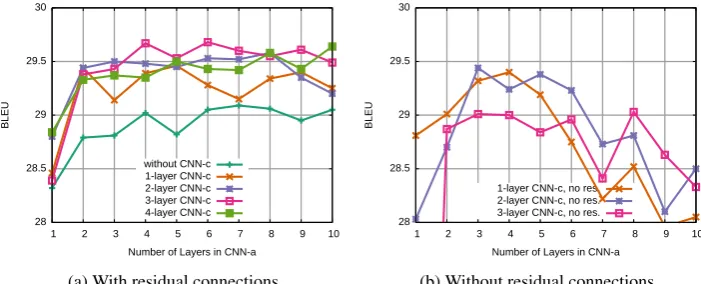
5.3 Convolutional Encoder Architecture Details
We next motivate our design of the convolutional
encoder (§3.2). We use the smaller IWSLT’14
German-English setup without unknown word re-placement to enable fast experimental turn-around. BLEU results are averaged over three training runs initialized with different seeds.
Figure2 shows accuracy for a different number
of layers of both CNNs with and without residual connections. Our first observation is that computing
the conditional inputcidirectly over embeddingse
(line ”withoutCNN-c”) is already working well at
28.3 BLEU with a single CNN-a layer and at 29.1
BLEU for CNN-a with 7 layers (Figure 2a).
In-creasing the number of CNN-clayers is beneficial
up to three layers and beyond this we did not ob-serve further improvements. Similarly, increasing
the number of layers inCNN-abeyond six does not
increase accuracy on this relatively small dataset. In general, choosing two to three times as many layers
in CNN-a as in CNN-c is a good rule of thumb.
Without residual connections, the model fails to utilize the increase in modeling power from addi-tional layers, and performance drops significantly
for deeper encoders (Figure2b).
Our convolutional architecture relies on two sets
of networks, CNN-a for attention score
computa-tion ai andCNN-c for the conditional input ci to
be fed to the decoder. We found that using the same network for both tasks, similar to recurrent encoders, resulted in poor accuracy of 22.9 BLEU. This compares to 28.5 BLEU for separate single-layer networks, or 28.3 BLEU when aggregating
embeddings forci. Increasing the number of layers
in the single network setup did not help. Figure2(a)
suggests that the attention weights (CNN-a) need
to integrate information from a wide context which can be done with a deep stack. At the same time,
the vectors which are averaged (CNN-c) seem to
benefit from a shallower, more local representation closer to the input words. Two stacks are an easy way to achieve these contradicting requirements.
In AppendixAwe visualize attention scores and
find that alignments for CNN encoders are less sharp compared to BiLSTMs, however, this does not affect the effectiveness of unknown word re-placement once we adjust for shifted maxima. In
Appendix B we investigate whether deep
convo-lutional encoders are required for translating long sentences and observe that even relatively shallow encoders perform well on long sentences.
5.4 Training and Generation Speed
For training, we use the fast CuDNN LSTM im-plementation for layers without attention and ex-periment on IWSLT’14 with batch size 32. The single-layer BiLSTM model trains at 4300 target words/second, while the 6/3 deep convolutional en-coder compares at 6400 words/second on an NVidia Tesla M40 GPU. We do not observe shorter over-all training time since SGD converges slower than Adam which we use for BiLSTM models.
We measure generation speed on an Intel Haswell CPU clocked at 2.50GHz with a single thread for BLAS operations. We use vocabulary selection which can speed up generation by up to a factor of ten at no cost in accuracy via making the time to
compute the final output layer negligible (Mi et al.,
2016;L’Hostis et al., 2016). This shifts the focus from the efficiency of the encoder to the efficiency
of the decoder. On IWSLT’14 (Table3a) the
convo-lutional encoder increases the speed of the overall model by a factor of 1.35 compared to the BiLSTM encoder while improving accuracy by 0.7 BLEU. In this setup both encoders models have the same hid-den layer and embedding sizes.
On the larger WMT’15 English-German task
(Table3b) the convolutional encoder speeds up
gen-eration by 2.1 times compared to a two-layer BiL-STM. This corresponds to 231 source words/second with beam size 5. Our best model on this dataset generates 203 words/second but at slightly lower accuracy compared to the full vocabulary setting in
Table2. The recurrent encoder uses larger
embed-dings than the convolutional encoder which were required for the models to match in accuracy.
The smaller embedding size is not the only
rea-son for the speed-up. In Table 3a (a), we
com-pare a Conv 6/3 encoder and a BiLSTM with equal embedding sizes. The convolutional encoder is still 1.34x faster (at 0.7 higher BLEU) although it requires roughly 1.6x as many FLOPs. We be-lieve that this is likely due to better cache locality for convolutional layers on CPUs: an LSTM with
fused gates7requires two big matrix multiplications
with different weights as well as additions, multi-plications and non-linearities for each source word, while the output of each convolutional layer can be computed as whole with a single matrix multiply.
For comparison, the quantized deep LSTM-7Our bi-directional LSTM implementation is
28 28.5 29 29.5 30
1 2 3 4 5 6 7 8 9 10
BLEU
Number of Layers in CNN-a without CNN-c 1-layer CNN-c 2-layer CNN-c 3-layer CNN-c 4-layer CNN-c
(a) With residual connections
28 28.5 29 29.5 30
1 2 3 4 5 6 7 8 9 10
BLEU
Number of Layers in CNN-a 1-layer CNN-c, no res. 2-layer CNN-c, no res. 3-layer CNN-c, no res.
[image:8.595.121.472.59.201.2](b) Without residual connections
Figure 2: Effect of encoder depth on IWSLT’14 with and without residual connections. The x-axis varies
the number of layers inCNN-aand curves show differentCNN-csettings.
Encoder Words/s BLEU
BiLSTM 139.7 22.4
Deep Conv. 6/3 187.9 23.1
(a) IWSLT’14 German-English generation speed on tst2013with beam size 10.
Encoder Words/s BLEU
2-layer BiLSTM 109.9 23.6 Deep Conv. 8/4 231.1 23.7 Deep Conv. 15/5 203.3 24.0
(b) WMT’15 English-German generation speed on new-stest2015with beam size 5.
Table 3: Generation speed in source words per second on a single CPU core using vocabulary selection.
based model in (Wu et al., 2016) processes 106.4
words/second for English-French on a CPU with 88 cores and 358.8 words/second on a custom TPU chip. The optimized RNNsearch model and C++
decoder described by (Junczys-Dowmunt et al.,
2016) translates 265.3 words/s on a CPU with a
similar vocabulary selection technique, computing 16 sentences in parallel, i.e., 16.6 words/s on a sin-gle core.
6 Conclusion
We introduced a simple encoder model for neu-ral machine translation based on convolutional net-works. This approach is more parallelizable than recurrent networks and provides a shorter path to capture long-range dependencies in the source. We find it essential to use source position embeddings as well as different CNNs for attention score com-putation and conditional input aggregation.
Our experiments show that convolutional en-coders perform on par or better than baselines based on bi-directional LSTM encoders. In comparison to other recent work, our deep convolutional en-coder is competitive to the best published results to date (WMT’16 English-Romanian) which are obtained with significantly more complex models (WMT’14 English-French) or stem from improve-ments that are orthogonal to our work (WMT’15 English-German). Our architecture also leads to
large generation speed improvements: translation models with our convolutional encoder can translate twice as fast as strong baselines with bi-directional recurrent encoders.
References
Dzmitry Bahdanau, Kyunghyun Cho, and Yoshua Ben-gio. 2015. Neural machine translation by jointly learning to align and translate. InProc. of ICLR. James Bradbury and Richard Socher. 2016. MetaMind
Neural Machine Translation System for WMT 2016. InProc. of WMT.
Mauro Cettolo, Jan Niehues, Sebastian St¨uker, Luisa Bentivogli, and Marcello Federico. 2014. Report on the 11th IWSLT evaluation campaign. In Proc. of IWSLT.
Kyunghyun Cho, Bart Van Merri¨enboer, Dzmitry Bah-danau, and Yoshua Bengio. 2014a. On the Properties of Neural Machine Translation: Encoder-decoder Ap-proaches. InProc. of SSST.
Kyunghyun Cho, Bart Van Merri¨enboer, Caglar Gul-cehre, Dzmitry Bahdanau, Fethi Bougares, Holger Schwenk, and Yoshua Bengio. 2014b. Learning Phrase Representations using RNN Encoder-Decoder for Statistical Machine Translation. In Proc. of EMNLP.
Junyoung Chung, Kyunghyun Cho, and Yoshua Bengio. 2016. A Character-level Decoder without Explicit Segmentation for Neural Machine Translation. arXiv preprint arXiv:1603.06147.
Ronan Collobert, Koray Kavukcuoglu, and Clement Farabet. 2011a. Torch7: A Matlab-like Environment for Machine Learning. InBigLearn, NIPS Workshop. http://torch.ch.
Ronan Collobert, Jason Weston, L´eon Bottou, Michael Karlen, Koray Kavukcuoglu, and Pavel Kuksa. 2011b. Natural Language Processing (almost) from scratch. JMLR12(Aug):2493–2537.
Chris Dyer, Victor Chahuneau, and Noah A Smith. 2013. A Simple, Fast, and Effective Reparameterization of IBM Model 2. Proc. of ACL.
Kaiming He, Xiangyu Zhang, Shaoqing Ren, and Jian Sun. 2015. Deep Residual Learning for Image Recog-nition. InProc. of CVPR.
Sepp Hochreiter and J¨urgen Schmidhuber. 1997. Long short-term memory. Neural computation9(8):1735– 1780.
S´ebastien Jean, Kyunghyun Cho, Roland Memisevic, and Yoshua Bengio. 2014. On Using Very Large Target Vocabulary for Neural Machine Translation. arXiv preprint arXiv:1412.2007v2.
S´ebastien Jean, Orhan Firat, Kyunghyun Cho, Roland Memisevic, and Yoshua Bengio. 2015. Montreal Neural Machine Translation systems for WMT15. In Proc. of WMT. pages 134–140.
Marcin Junczys-Dowmunt, Tomasz Dwojak, and Hieu Hoang. 2016. Is Neural Machine Translation Ready for Deployment? A Case Study on 30 Translation Di-rections.arXiv preprint arXiv:1610.01108.
Nal Kalchbrenner and Phil Blunsom. 2013. Recurrent Continuous Translation Models. InProc. of EMNLP. Nal Kalchbrenner, Lasse Espeholt, Karen Simonyan, Aaron van den Oord, Alex Graves, and Koray Kavukcuoglu. 2016. Neural Machine Translation in Linear Time. arXiv.
Diederik P. Kingma and Jimmy Ba. 2014. Adam: A Method for Stochastic Optimization. Proc. of ICLR. Philipp Koehn, Hieu Hoang, Alexandra Birch, Chris
Callison-Burch, Marcello Federico, Nicola Bertoldi, Brooke Cowan, Wade Shen, Christine Moran, Richard Zens, Chris Dyer, Ondej Bojar, Alexandra Constantin, and Evan Herbst. 2007. Moses: Open Source Toolkit for Statistical Machine Translation. In Proc. of ACL.
Andrew Lamb and Michael Xie. 2016. Con-volutional Encoders for Neural Machine Trans-lation. https://cs224d.stanford.edu/
reports/LambAndrew.pdf. Accessed:
2010-10-31.
Gurvan L’Hostis, David Grangier, and Michael Auli. 2016. Vocabulary Selection Strategies for Neural Ma-chine Translation. arXiv preprint arXiv:1610.00072. Minh-Thang Luong, Hieu Pham, and Christopher D Manning. 2015a. Effective approaches to attention-based neural machine translation. In Proc. of EMNLP.
Minh-Thang Luong, Ilya Sutskever, Quoc V Le, Oriol Vinyals, and Wojciech Zaremba. 2015b. Addressing the Rare Word Problem in Neural Machine Transla-tion. InProc. of ACL.
Fandong Meng, Zhengdong Lu, Mingxuan Wang, Hang Li, Wenbin Jiang, and Qun Liu. 2015. Encoding Source Language with Convolutional Neural Network for Machine Translation. InProc. of ACL.
Haitao Mi, Zhiguo Wang, and Abe Ittycheriah. 2016. Vocabulary Manipulation for Neural Machine Trans-lation.arXiv preprint arXiv:1605.03209.
Razvan Pascanu, Tomas Mikolov, and Yoshua Bengio. 2013. On the Difficulty of Training Recurrent Neural Networks.ICML (3)28:1310–1318.
Ngoc-Quan Pham, Germn Kruszewski, and Gemma Boleda. 2016. Convolutional Neural Network Lan-guage Models. InProc. of EMNLP.
Marc’Aurelio Ranzato, Sumit Chopra, Michael Auli, and Wojciech Zaremba. 2015. Sequence level Train-ing with Recurrent Neural Networks. In Proc. of ICLR.
Holger Schwenk. 2014. http://www-lium. univ-lemans.fr/˜schwenk/cslm_joint_
paper/. Accessed: 2016-10-15.
Rico Sennrich, Barry Haddow, and Alexandra Birch. 2016b. Neural Machine Translation of Rare Words with Subword Units. InProc. of ACL.
Nitish Srivastava, Geoffrey E. Hinton, Alex Krizhevsky, Ilya Sutskever, and Ruslan Salakhutdinov. 2014. Dropout: a simple way to prevent Neural Networks from overfitting. JMLR15:1929–1958.
Sainbayar Sukhbaatar, Jason Weston, Rob Fergus, and Arthur Szlam. 2015. End-to-end Memory Networks. InProc. of NIPS. pages 2440–2448.
Ilya Sutskever, Oriol Vinyals, and Quoc V Le. 2014. Se-quence to SeSe-quence Learning with Neural Networks. InProc. of NIPS. pages 3104–3112.
Zhaopeng Tu, Baotian Hu, Zhengdong Lu, and Hang Li. 2015. Context-dependent Translation selection us-ing Convolutional Neural Network. InProc. of ACL-IJCNLP.
Yonghui Wu, Mike Schuster, Zhifeng Chen, Quoc V Le, Mohammad Norouzi, Wolfgang Macherey, Maxim Krikun, Yuan Cao, Qin Gao, Klaus Macherey, et al. 2016. Google’s Neural Machine Translation Sys-tem: Bridging the Gap between Human and Machine Translation. arXiv preprint arXiv:1609.08144.
Zichao Yang, Zhiting Hu, Yuntian Deng, Chris Dyer, and Alex Smola. 2016. Neural Machine Translation with Recurrent Attention Modeling. arXiv preprint arXiv:1607.05108.
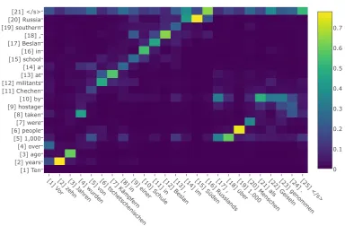
A Alignment Visualization
In Figure 4 and Figure 5, we plot attention
scores for a sample WMT’15 English-German and WMT’14 English-French translation with BiLSTM and deep convolutional encoders. The translation is on the x-axis and the source sentence on the y-axis. The attention scores of the BiLSTM output are sharp but do not necessarily represent a correct alignment. For CNN encoders the scores are less focused but still indicate an approximate source
lo-cation, e.g., in Figure 4b, when moving the clause
”over 1,000 people were taken hostage” to the back of the translation. For some models, attention max-ima are consistently shifted by one token as both in
Figure4band Figure5b.
Interestingly, convolutional encoders tend to
fo-cus on the last token (Figure4b) or both the first and
last tokens (Figure5b). Motivated by the
hypothe-sis that the this may be due to the decoder depend-ing on the length of the source sentence (which it cannot determine without position embeddings), we explicitly provided a distributed representation of the input length to the decoder and attention mod-ule. However, this did not cause a change in atten-tion patterns nor did it improve translaatten-tion accuracy.
B Performance by Sentence Length
20 21 22 23 24 25 26 27 28 29
1-7 7-9 9-11 11-13 13-15 15-17 17-19 19-21 21-23 23-26 26-28 28-31 31-35 35-43 43-85
BLEU
Range of Sentence Lengths
[image:11.595.68.288.448.532.2]2-layer BiLSTM Deep Conv. 6/3 Deep Conv. 8/4 Deep Conv. 15/5
Figure 3: BLEU per sentence length on WMT’15
English-German newstest2015. The test set is
par-titioned into 15 equally-sized buckets according to source sentence length.
One characteristic of our convolutional encoder architecture is that the context over which outputs are computed depends on the number of layers. With bi-directional RNNs, every encoder output
de-pends on the entire source sentence. In Figure 3,
we evaluate whether limited context affects the translation quality on longer sentences of WMT’15 English-German which often requires moving verbs
over long distances. We sort the newstest2015test
set by source length, partition it into 15 equally-sized buckets, and compare the BLEU scores of
models listed in Table2on a per-bucket basis.
There is no clear evidence for sub-par transla-tions on sentences that are longer than the observ-able context per encoder output. We include a small
encoder with a 6-layerCNN-cand a 3-layerCNN-a
[1] V or
[2] z ehn
[3] Ja hr
en [4] wur
den [5] mehr[6] a
ls [7] 1
.000 [8] M
ensc hen [9] v
on [1 0] ts chet sc heni sc hen [1 1] Kä mpfer n [1
2] in[13] ei ner [1
4] Schul e [1
5] in[16] Besl an [1 7] a ls [1 8] Gei sel n [1
9] genommen[20] .[21] </ s> [1] Ten [2] years [3] ago [4] over [5] 1,000 [6] people [7] were [8] taken [9] hostage [10] by [11] Chechen [12] militants [13] at [14] a [15] school [16] in [17] Beslan [18] , [19] southern [20] Russia [21] </s> 0 0.2 0.4 0.6 0.8
(a) 2-layer BiLSTM encoder.
[1] V or [2] z
ehn [3] Ja
hr en [4] wur
den [5] v
on [6] ts
chet sc
heni sc
hen [7] Kä
mpfer n [8
] in[9] ei ner [1
0] Schul e [1
1] i[1n2] Besl an [1
3] ,[14] i[1m5] Süden[16] R us
slands [1
7] ,[18] über[19] 1 .000 [2 0] M ensc hen [2
1] a[2ls2] Gei sel
n [2
3] genommen[24] .[25] </ s> [1] Ten [2] years [3] ago [4] over [5] 1,000 [6] people [7] were [8] taken [9] hostage [10] by [11] Chechen [12] militants [13] at [14] a [15] school [16] in [17] Beslan [18] , [19] southern [20] Russia [21] </s> 0 0.1 0.2 0.3 0.4 0.5 0.6 0.7
[image:12.595.103.488.418.670.2](b) Deep convolutional encoder with 15-layer CNN-a and 5-layer CNN-c.
[1] La[2] pol ice [3] de[4] Phuk
et [5] a[6
] inter rogé [7
] les[8] <unk>[9] penda nt [1
0] deux[11] j our
s [1
2] a vant [1
3] de[14] fa ire [1
5] la[16] fa br
ica tion [1
7] de[18] l'[19] hi stoi
re [2
0] .[21] </ s> [1] Phuket
[2] police [3] interviewed [4] Bamford [5] for [6] two [7] days [8] before [9] she [10] confessed [11] to [12] fabricating [13] the [14] story [15] . [16] </s>
0 0.2 0.4 0.6 0.8
(a) 2-layer BiLSTM encoder.
[1] La[2] pol ice
[3] de[4] Phuk
et [5] a [6
] inter rogé [7] <unk>[8] penda
nt [9] deux[1
0] j our
s [1
1] a vant
[1 2] d'[13] a
voir [1 4] a
voué [1
5] l'[16] hi st
oire [1
7] .[18] </ s>
[1] Phuket [2] police [3] interviewed [4] Bamford [5] for [6] two [7] days [8] before [9] she [10] confessed [11] to [12] fabricating [13] the [14] story [15] . [16] </s>
0 0.1 0.2 0.3 0.4 0.5 0.6
[image:13.595.99.488.133.647.2](b) Deep convolutional encoder with 20-layer CNN-a and 5-layer CNN-c.