Munich Personal RePEc Archive
Euro Area and U.S. External
Adjustment: The Role of Commodity
Prices and Emerging Market Shocks
Giovannini, Massimo and Hohberger, Stefan and Kollmann,
Robert and Ratto, Marco and Roeger, Werner and Vogel,
Lukas
European Commission, Joint Research Centre, European
Commission, Joint Research Centre, ECARES, Université Libre de
Bruxelles and CEPR, European Commission, Joint Research Centre,
European Commission, DG ECFIN, European Commission, DG
ECFIN
6 August 2018
Online at
https://mpra.ub.uni-muenchen.de/88664/
1
Euro Area and U.S. External Adjustment:
The Role of Commodity Prices and Emerging Market Shocks
August 6, 2018
Massimo Giovannini (European Commission, Joint Research Centre) Stefan Hohberger (European Commission, Joint Research Centre) Robert Kollmann (ECARES, Université Libre de Bruxelles and CEPR)(*)
Marco Ratto (European Commission, Joint Research Centre) Werner Roeger (European Commission, DG ECFIN)
Lukas Vogel (European Commission, DG ECFIN)
The trade balances of the Euro Area (EA) and of the US have improved markedly after the Global Financial Crisis. This paper quantifies the drivers of EA and US economic fluctuations and external adjustment, using an estimated (1999-2017) three-region (US, EA, rest of world) DSGE model with trade in manufactured goods and in commodities. In the model, commodity prices reflect global demand and supply conditions. The paper highlights the key contribution of the post-crisis collapse in commodity prices for the EA and US trade balance reversal. Aggregate demand shocks originating in Emerging Markets too had a significant impact on EA and US trade balances. The broader lesson of this paper is that Emerging Markets and commodity shocks are major drivers of advanced countries’ trade balances and terms of trade.
JEL Codes: F2,F3,F4
Keywords: EA and US external adjustment, commodity markets, emerging markets.
(*)
2
1. Introduction
Since the early 2000s, the world economy has experienced major changes. Emerging economies
grew rapidly, and their share in world output increased steadily. Both the US and the Euro Area
(EA) experienced a boom-bust cycle. These developments have been accompanied by substantial
trade balance adjustments. In the first half of the 2000s, the US trade balance deteriorated
markedly, reaching about -6% of GDP in 2005-7, while the EA trade balance fluctuated around
zero. After the Global Financial Crisis (2007-8), the EA and US trade balances both rose
noticeably: the US trade deficit fell markedly, while the EA has been running steadily increasing
trade balance surpluses.
This raises a number of questions: Has the EA/US boom-bust cycle been a major driver
of global imbalances, or has the growth divergence between the rest of the world (RoW) and the
EA/US shaped trade balances more strongly? A possible explanation for the widening pre-crisis
US trade deficit is also provided by the saving glut hypothesis (Bernanke (2005)) which
highlights the fact that rapid growth in the RoW has been associated with high RoW saving rates
(perhaps due to heightened risk aversion as a consequence of the Asian financial crisis of the late
1990s). Thus high saving in the RoW may have outweighed the effect of high RoW productivity
growth on the RoW external balance. A further factor (e.g., stressed by McKibbin and Stoeckel
(2018)) that might help explain the trade balance facts, are the spectacular commodity price
fluctuations during the last two decades: commodity prices rose sharply before the Global
Financial Crisis, and collapsed afterwards. This might have contributed to the pre-crisis
worsening of the US trade balance, and the EA and US post-crisis trade balance reversal. Note,
however, that this factor is only partly independent from the other mechanisms mentioned above,
since commodity prices may themselves be affected by the global business cycle.
To quantitatively evaluate the role of these mechanisms and forces, we develop a rich
three-region New Keynesian DSGE (Dynamic Stochastic General Equilibrium) model of the
world economy that includes a commodity sector. We estimate that model (with Bayesian
Methods), using 1999q1-2017q2 data for the EA, US and an aggregate of rest of the world
(RoW) countries. The use of a rich estimated model allows us to identify periods dominated by specific shocks. In the model, commodity prices endogenously respond to global macroeconomic
conditions. However, commodity prices are also driven by commodity-specific supply and
demand shocks that may, e.g., reflect the discovery of new oil fields, or changes in the
commodity intensity of the manufacturing sector.
3
activity and of external imbalances. According to our estimates, the EA and US pre-crisis booms
were mainly driven by positive domestic aggregate demand shocks. Our findings suggest that
those shocks contributed to the widening pre-crisis trade deficit in the US, and also had a
negative influence on the EA trade balance. The RoW growth divergence, which accelerated in
the 2000s, was mainly driven by strong positive RoW aggregate supply (productivity) shocks;
those RoW shocks only had a muted effect on EA and US trade balances. However, before the
crisis, adverse aggregate demand shocks in RoW, driven by a rise in private saving rates, had a
noticeable negative influence on EA and US trade balances. Our findings are thus consistent with
a pre-crisis ‘saving glut’ effect (Bernanke (2005)) for both US and EA trade balances. We also
find that positive commodity-specific demand shocks during the pre-crisis boom had a marked
negative effect on EA and US trade balances.
As pointed out above, EA and US trade balances improved strongly after the Global
Financial Crisis. This is often viewed as reflecting weak domestic aggregate demand. This paper
provides a nuanced assessment of that view. In particular, we argue that commodity shocks
played an important role for the post-crisis EA and US trade balance reversal. In the US, where
the post-crisis slump and the contraction of aggregate demand was more short-lived than in the
EA (see analysis in Kollmann et al (2016)), a major expansion of domestic commodity
production and a fall in demand for imported commodities stabilized the trade deficit at a lower
level, after the financial crisis. Similarly in the EA, negative shocks to commodity import demand
contributed markedly to the post-crisis trade balance improvement. However, the post-crisis
weakness of EA aggregate demand, and the depreciation of the Euro, also played a significant
part in the EA trade balance reversal. Positive RoW aggregate demand shocks during the
post-crisis period too contributed to the US and EA trade balance improvements. The broader lesson
of this paper is thus that Emerging Markets (RoW) and commodity shocks are key drivers of
advanced countries’ trade balances and terms of trade.
The trade balance developments discussed in this paper have some parallels in the
external adjustments triggered by the oil shocks of the 1970s; those shocks triggered a sharp rise
in the trade balances of oil exporters, and a trade balance deterioration of the groups of advanced
and (especially) non-fuel developing countries (Obstfeld and Rogoff (1996)). An important
difference between the global macroeconomic environment of the 2000s and that of the 1970s, is
that the 2000s saw massive growth in Emerging Markets, which suggests that the commodity
price hikes of the 2000s might have been driven more by expanding demand for commodities,
4
Quantitative analyses of oil and commodity price fluctuations mostly rely on
reduced-form statistical models, such as vector auto regressions (see, e.g., Kilian (2009), Kilian et al.
(2009), Peersman and Van Robays (2009), ECB (2010), Caldara et al. (2017)), or on
semi-structural models (e.g., Dieppe et al. (2018)). With few exceptions, semi-structural (DSGE) open
economy models abstract from international trade in commodities. Existing DSGE models with
commodity trade often assume a small open economy that faces exogenous commodity prices
(e.g., Miura (2017)). By contrast, the paper here develops (and estimates) a multi-country DSGE
model with endogenous commodity prices. The paper here is closest to Forni, Gerali, Notarpietro and Pisani (2015), who estimate a two-country DSGE model of the EA and the non-EA rest-of-the-world, using data for 1995-2012.1 Our model differs from that work in that we use a rich
three-region model (EA, US, RoW) that allows us to analyze the noticeable differences between the dynamics of the EA and US external accounts. Our paper focuses on the interaction between
the three regions, and we use a sample period that includes the post-2014 commodity price
collapse.2 We document the key role of the expansion of US commodity production during the
2010s for the improvement in the US trade balance, during that period.
2. EA, US and RoW macroeconomic conditions and external adjustment, 1999-2017
This paper studies macroeconomic developments and linkages in the EA, US and an aggregate of
the rest of the world (RoW).3 Figures 1-3 show time series for EA, US and RoW GDP and trade
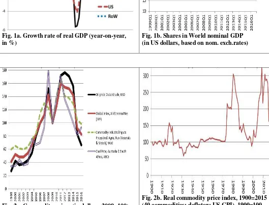
flows, since 1999. Fig.1a documents that real GDP growth has been markedly higher in RoW
than in the EA and the US. The mean real GDP growth rates of the three regions in 1999-2016
were 1.3% (EA), 1.9% (US) and 3.6% (RoW) per annum, respectively. As a result of this growth
differential, the share of RoW GDP in total world GDP has increased steadily, from close to 40%
(1999) to more than 50% (2016); see Fig. 1b. During the Great Recession (2008-9), GDP
contracted in all three regions, but the contraction was milder in RoW than in the EA and US. In
2009-11, RoW growth rebounded to pre-crisis growth rates, and then declined somewhat. EA and
US GDP growth too rebounded in 2009-11, but remained below pre-crisis growth rates. After the
1
Simpler multi-country DSGE simulation models of the role of energy for international adjustment have been developed by Sachs (1981), McKibbin and Sachs (1991), Backus and Crucini (2000) and Gars and Olovsson (2018) and Bornstein al. (2018).
2
Forni et al. (2015) analyze the effects of oil shocks; by contrast, the paper here considers shocks to a broader bundle of commodities.
3
5
eruption of the Southern European sovereign debt crisis (2011), the EA experienced a recession
(2012-13).
These divergent GDP trends and uncoupled cycles were accompanied by dramatic
fluctuations in commodity prices, and by major shifts in the three regions’ trade balances. The
prices of a wide range of commodities rose sharply during the early 2000s, until the Global
Financial Crisis. This is documented in Fig. 2a, where oil and coal prices as well as two global
commodity price indices (in US dollars) are plotted. Note, e.g., that the oil price was multiplied
by a factor greater than 5 between 1999 and 2008. Commodity prices contracted sharply during
the financial crisis, but rebounded strongly after the crisis; commodity prices then fell again
sharply (by more than 50%) after 2011. To put these developments into a long-run perspective,
Fig. 2b plots an index of real prices (deflated by the US CPI) of 40 commodities for the period
1900-2015, constructed by Jacks (2013, 2016). The magnitude of the recent commodity price
boom-bust cycle is only comparable to the 1973-86 commodity boom-bust cycle; it dwarfs all
other commodity cycles since 1900.
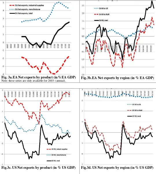
EA net exports of goods (merchandise) fluctuated around zero before the crisis, and then
rose steadily, reaching about 2.5% of EA GDP in 2016 (see Fig. 3b). Note that all data on trade
flows used in this paper pertain to goods trade, as there are no time series for bilateral services
trade, between the three regions (EA, US, RoW).4 By contrast to the EA, the US has been
running a sizable trade deficit (goods) during the whole sample period (in fact, since the
mid-1980s). The US trade deficit peaked at about 6% of GDP in 2005-07 (see Fig. 3c). The trade
deficit has fallen after the financial crisis, to about 4% of US GDP in 2017.
To understand whether/how these trade balance reversals might be linked to the
commodity boom-bust cycle and the decoupled regional growth trends, we also plot EA and US
net exports that are disaggregated by trade partner (regions), and by product (all net exports series
are normalized by GDP); see Fig.3. Specifically, we disaggregate trade flows (goods) into:
(i) ‘industrial supplies and materials’, (henceforth referred to as ‘industrial supplies’), a broad
basket of commodities comprising petroleum, mineral products and other raw materials; (ii) an
aggregate of all other products, henceforth referred to as ‘manufactures’.5
4
The EA and (especially) the US are running a net surplus for trade in services. However, the services trade surplus is smaller than the goods trade balance, and much more stable. The goods trade balance is thus highly positively correlated with the total (goods and services) trade balance.
5
6
The disaggregation of net exports by trade partners shows that the EA has been running a
small and relatively stable trade balance surplus (ranging between about 0.5% and 1% of EA
GDP) against the US, since 1999. Thus, trade with RoW drives the major swings in EA and US
total net exports (see Figs. 3b and 3d). Trade with RoW also accounts for the lion share of EA
and US gross trade flows. Manufactures account for more than 70% of EA bilateral gross trade with RoW, and for about 60% of bilateral US-RoW trade.6
The EA had a trade balance surplus for manufactures, and a trade deficit for industrial
supplies, in 1999-2016 (see Fig. 3a). EA net exports of manufactures increased steadily until
2013, and then declined somewhat. EA net imports of industrial supplies rose before the crisis,
fell somewhat during the crisis, then rose again (2010-11), and fell substantially thereafter. EA
net imports of industrial supplies thus track closely the commodity price cycle (see above). The
overall EA trade balance (across all products and trade partners) comoves closely with the EA’s
industrial supplies trade balance--the overall trade balance and the industrial supplies trade
balance both improved markedly after 2012.
The US has been running a persistent trade deficit, for manufactures and for industrial supplies. The dynamics of US net imports of industrial supplies too tracks the evolution of
commodity prices. Net imports of industrial supplies have fallen more in the US than in the EA,
after the financial crisis. Note that the US is a major producer and exporter of oil and other
commodities, while the EA is a negligible producer/exporter of commodities. US crude oil
production doubled between 2010 and 2015, driven by the expansion of oil shale extraction
(Baffes et al. (2015)). This may have contributed to the sharper fall in US net commodity
imports. Interestingly, US net imports of manufactures have followed an opposite trend (than US
net commodity imports) and increased noticeably, after the crisis.
This overview of the historical data suggests that commodity shocks may have
contributed to the post-crisis reversal of EA and US trade balances. Below, we use an estimated
DSGE model to quantify the contribution of the commodity cycle to EA and US external
balances, and we disentangle the influence of commodity-specific shocks from other drivers,
such as aggregate demand and supply shocks.
‘industrial supplies’. Importantly, EA exports and imports exclude intra-EA trade. EA and US trade flows to/from RoW represent flows to/from all countries other than the US and the EA.
6
7
3. Model description
We develop a model of a three-region world consisting of the EA, US and RoW. The three
regions are linked via trade in goods and a financial asset. The EA and US blocks of the model
are fairly rich; both blocks have the same structure (but model parameters are allowed to differ
across these two regions). The RoW block of the model is simpler (fewer shocks). In all three
regions, economic decisions are made by forward-looking households and firms; each region
exhibits nominal and real rigidities, and is buffeted by a range of supply and demand shocks, as
in standard New Keynesian DSGE models. A key difference between the regions is that the
model postulates that only RoW produces commodities. Thus, in the model, all commodities used
by the EA and US are imported from RoW.
The EA and US model blocks assume two (representative) infinitely-lived households,
firms and a government. EA and US households provide labor services to domestic firms. One of
the two households in each region has access to financial markets, and she owns her region’s
production capital and firms. The other household has no access to financial markets, does not
own assets, and each period consumes her disposable wage and transfer income. We refer to
these two agents as ‘Ricardian’ and ‘hand-to-mouth’ households, respectively.
In each region, a final good is produced by perfectly competitive firms that use local
intermediate goods and imported commodities and manufactured goods as inputs. Intermediates
are produced by monopolistically competitive firms using local labor and capital. Wage rates are
set by monopolistic trade unions. Nominal intermediate good prices and nominal wages are
sticky. Governments purchase the local final good, make lump-sum transfers to local households,
levy labor and consumption taxes and issue domestic debt. All exogenous random variables
follow independent autoregressive processes.
We next present the key aspects of the EA model block. As mentioned above, the US
block has a symmetric structure. The RoW block is described in Section 3.5. 7
3.1. EA households
A household’s welfare depends on consumption and hours worked. EA household i=r,h (r : Ricardian, h: hand-to-mouth) has the period utility function
1 1 1 1 1
1 1
1 ( ) ( ) 1 ( )
N N
i i C i N i i N i
t t t t t t t
U ≡ −θ C −η C− −θ −s ⋅ C −θ +θ N −η N− +θ ,
7
8 with 0<
θ θ
, ,NstN and 0<η η
C, N<1. it
C andNti are consumption and the labor hours of household
i in period t, respectively. We assume (external) habit formation for consumption and labor
hours.8 stN is an exogenous shock to the disutility of labor. Household behavior at date t seeks to
maximize expected life-time utility at that date, Vti, defined by Vti= +U Eti tβt t, 1+Vti+1,where
, 1
0<
β
t t+<1 is a subjective discount factor that fluctuates exogenously.The EA Ricardian household owns all domestic firms, and holds domestic government
bonds (denominated in local currency and not traded internationally) and internationally traded
bonds. Her period t budget constraint is:
(1+
τ
C)PCt tr+Btr+1 = −(1τ
N)W Nt tr +Btr(1+ +itr) divt+Ttr,where P W divt, t, t and Ttr are the consumption (final good) price, the nominal wage rate,
dividends generated by domestic firms, and government transfers received by the Ricardian
household. Btr+1 denotes the Ricardian household’s total bond holdings at the end of period t, and
r t
i is the nominal return on the household’s bond portfolio between periods t-1 and t. τ C and τN
are (constant) consumption and labor tax rates, respectively.
The hand-to-mouth household does not trade in asset markets and simply consumes her
disposable wage and transfer income. Her budget constraint is: (1+
τ
C)PCt th = −(1τ
N)W Nt th+Tth.3.2. EA technology and firms
EA production is a multi-stage process. In the first stage, monopolistically competitive EA firms
use domestic capital and labor to produce non-tradable differentiated intermediate goods.
Perfectly competitive EA firms then combine domestic intermediates, imported commodities and
imported manufactured goods to produce a final good that is used for domestic private and
government consumption, investment and exports.
3.2.1. EA intermediate goods sector
In the EA, there is a continuum of intermediate goods indexed by j∈[0,1]. Each good is
produced by a single firm. All EA intermediate good firms face identical decision problems. Firm
j has technology ytj=Θt(Ntj) (α cu Ktj tj)1−α, where y N K cutj, tj, tj, tj are the firm’s output, labor input,
8
To allow for balanced growth, the disutility of labor features the multiplicative term 1
( h) ;
t
9
capital stock and capacity utilization, respectively. Total factor productivity (TFP) Θ >t 0 is
exogenous and common to all EA intermediate good producers. Log TFP is the sum of a
stationary autoregressive process and of a unit root process whose first difference is highly
serially correlated.
The law of motion of firm j’s capital stock is Kt+j1=Ktj(1− +
δ
) Itj, with 0< <δ 1; Itj is grossinvestment. The period t dividend of intermediate good firm j is divtj=p y W Ntj tj− t tj−P ItK tj−Ptκtj,
where ptj and PtK are the price charged by the firm and the price of production capital,
respectively. At t, each intermediate good firm faces a downward sloping demand curve for her
output, with exogenous price elasticity
ε
t>1 that equals the substitution elasticity betweendifferent intermediate good varieties (see below). The firm bears a real cost
2 1
1
2 ( (1 ) ) /
j j j j
t pt pt pt
κ
≡γ
− +π
− of changing her price, whereπ
is the steady state inflation rate.The quadratic price adjustment cost implies that the inflation rate of local intermediates
1
ln( /j j ) t p pt t
π
≡ − obeys an expectational Phillips curve, up to a linear approximation:1 1
( ) j( / j ).
t Et t MC pt t
ε ε
π π β π π ϑ
−+
− = − + − Here MCtj is the marginal cost of intermediate good firms
and (ε−1)/ε is the inverse of the steady state mark-up factor.
β
is the steady state subjectivediscount factor of intermediate good firms, and
ϑ
j>
0
is a coefficient that depends on the cost ofchanging prices.
3.2.2. EA final good sector
The EA final good ( )Ot is produced from domestic and imported inputs, using the technology
1/ ( 1)/ 1/ ( 1)/ /( 1)
(( ) ( )d o o o (1 d) (o ) o o)o o ,
t t t t t
O= s ν D ν− ν + −s ν M ν− ν ν ν− with home bias parameter 0.5< <std 1 and substitution
elasticity 0.νo> Mt is a composite of the manufactured goods imported by EA (from US and
RoW). Dt ((1 stis) ( )1/ dYt (d1)/d ( ) ( )stis1/d ISt (d1)/d)d/(d1),
ν ν − ν ν ν− ν ν ν−
= − + withνd>0, is a CES aggregate of EA real
domestic value added, ,Yt and industrial supplies ISt (energy and non-energy commodities)
imported from RoW. 1 ( 1)/ /( 1)
0
{ ( j) t t }t t
t
t y dj
Y≡
∫
ε− ε ε ε− isan aggregateofthe local intermediates (see 3.2.1).The CES-weight attached to commodities,0< <stis 1,is an exogenous random variable that captures
10
a ‘commodity-specific demand shock’, because sist has a direct effect on commodity demand.
Note that EA commodity demand obeys ISt=( /(1stis −stis))× ×Yt (P Ptis/ ty)−νd. A fall in stis (reduction in
commodity intensity) lowers EA commodity demand, for given values of Yt and of the real
commodity price P Ptis/ ty (where is t
P and Pty are the prices of ISt and ,Yt respectively).
The price (=marginal cost) of the EA final good is Pt=( (s Ptd td)1−νO+ −(1 std)(Ptm)1−νO)1/(1−νO),
where 1 1 1/(1 )
((1 )( ) d ( ) d) d
d is y is is
t t t t t
P = −s P −ν +s P −ν −ν while Ptm is the import price index.
The EA final good Ot is used for domestic private and government consumption, for
investment and for exports.
3.2.3. EA export sector
There is a monopolistically competitive EA export sector. Firm in that sector purchase and
‘differentiate’ the EA final good, and then sell it to foreign final good firms. Like intermediate
good producers (see above), exporters face price adjustment costs. We assume that a fraction of
EA exporters sets prices in Euro (producer currency price setting, PCP). The remaining exporters
set prices in destination currency (pricing to market, PTM); see Betts and Devereux (2000). We
estimate the share of each region’s export firms that use PTM.
3.2.4. EA capital goods sector
New production capitalis generated using the domestic final good. Let Ξ ⋅t
ξ
( )It be the amount ofEA final good needed to produce It units of EA capital.
ξ
is an increasing, strictly convexfunction, while Ξt is an exogenous shock. The price of production capital is PtK=Ξt
ξ
'( ) .I Pt t3.3. Wage setting in the EA
We assume a monopolistic EA trade union that ‘differentiates’ homogenous EA labor hours
provided by the two domestic households into imperfectly substitutable labor services; the union
then offers those services to local intermediate good firms; the labor input Nt in those firms’
production functions is a CES aggregate of these differentiated labor services. The union sets
wage rates at a mark-up over the marginal rate of substitution between leisure and consumption.
The wage mark-up is inversely related to the degree of substitution between labor varieties in
11
3.4. EA monetary and fiscal policy
The EA monetary policy (nominal) interest rate it+1 is set at date t by the EA central bank
according to the interest rate feedback rule
1
1 (1 ) (1 )[ { ln( /4 4) } ]
i i i Y gap i
t t t t t t
i+ = −ρ i+ρ i + −ρ ηπ P P− −π η+ Y +ε ,
where Ytgapis the EA output gap, i.e. the (relative) deviation of actual GDP from potential GDP;9
i t
ε
is a white noise disturbance. EA real government consumption, Gt,is set according to the rule1
( )
G G G G G G
t t t
c − =c ρ c−−c +ε , where ctG≡PG P Yt t/( ty t) is government consumption normalized by
domestic value added. EA government transfers to households follow a feedback rule that links
transfers to the government budget deficit and to government debt.
3.5. The RoW block
As mentioned above, the RoW model block has a simplified structure. Specifically, the RoW
block consists of a budget constraint for the representative (Ricardian) household, demand
functions for domestic and imported inputs (derived from a CES final good aggregator), a New
Keynesian Phillips curve, and a Taylor rule for monetary policy. The RoW production structure
for manufactures is analogous to that of the EA and US, except that we assume that RoW does
not use physical capital, and so there is no physical investment in RoW.10
In RoW, a competitive sector supplies two distinct commodities (indexed using
superscript ‘c’), namely energy and non-energy materials, to domestic and foreign final good
firms.11 Commodity prices are flexible. The commodity supply price denominated in RoW
currency, c , RoW t
P , normalized by the RoW GDP deflator, y ,
RoW t
P , is an increasing function of RoW
commodity production,IStc: ln( ,/ ,) ln( )
c y c c
RoW t RoW t t t
P P = ×η IS −ε , where εtc is a disturbance that
9
Date t potential GDP is defined as GDP that would obtain under full utilization of the date t capital stock and steady state hours worked, if TFP equaled its trend (unit root) component at t.
10
Our data set includes GDP data for RoW, but RoW investment (and consumption) data are not available. The RoW model block assumes domestic frictions (habit formation) and external frictions (foreign bond holding costs) that might give the model sufficient flexibility to capture the empirical dynamics of RoW absorption, despite the fact that the theoretical setup abstracts from RoW physical investment.
11
12
captures exogenous commodity supply shocks (such as the discovery of new raw material
deposits). The parameter ηIS is the inverse of the price elasticity of commodity supply.12
EA, US and RoW demand for commodities is determined by final good producers in these
regions. US and RoW demand functions for commodities are analogous to the EA demand
function shown in Sect. 3.2.2. However, we assume that the commodity intensity of RoW final
good production is constant, i.e. there are no stochastic RoW commodity-specific demand
shocks. This assumption is made because we lack data on RoW commodity production and on
RoW commodity demand. Therefore, a RoW commodity-specific demand shock is not identified
in our empirical model. By contrast, identification of the EA and US commodity-specific demand
shocks is possible, as the model estimation uses volume and price data on commodity imports by
EA and US from RoW.
Empirically, the EA and US commodity import price indices differ (but are highly
positively correlated). To account for those differences (which may reflect different commodity
import mixes), we assume that competitive RoW export firms bundle energy and non-energy
commodities into destination-specific CES commodity aggregates. The ‘commodity supply
shocks’ discussed in the historical shock decompositions below (see Sect. 5.3) include the shocks
to RoW commodity supply schedules ( ),c t
ε as well as disturbances to the destination-specific
RoW commodity export bundles.
In RoW, there are also shocks to labor productivity, the subjective discount rate, the
relative preference for domestic versus imported manufactured goods, and to monetary policy.
3.6. International financial markets
The only internationally traded asset (held by Ricardian households) is a one-period bond
denominated in RoW currency.13 Ricardian households face a small quadratic cost associated
with their net foreign bond holdings (normalized by nominal GDP) from a target value (that cost
is rebated to the households in a lump sum fashion). This implies that foreign vs. domestic
interest rate spreads depend on foreign bond holdings (see Kollmann (2002, 2004)). E.g., the
12
We experimented with variants of the commodity supply schedule that also included lagged quantities (IS) on the right-hand side, to allow the short-run price elasticity to differ from the long-run elasticity. The coefficients of lagged quantities were insignificant, and short- and long-run supply elasticities were not significantly different. Also, the implied model dynamics was unaffected. In what follows, we thus use the simple static commodity supply equation shown above.
13
13
first-order conditions of the EA Ricardian household for domestic and international bonds yield
this modified EA uncovered interest parity (UIP) condition, up to a log-linear
approximation:iROW t, 1++E ln(t eEA tROW, 1+/eEA tROW, )= +it+1 αbbt+1+εtb, 0, b
α > where iROW t, 1+ and it+1 are RoW
and domestic interest rates at date t, ROW, EA t
e is the EA-RoW exchange rate (Euro per unit of RoW
currency), and bt+1 is the EA’s foreign bond position (normalized by GDP). εtb is an exogenous
shock to the cost of holding foreign bonds, referred to as a ‘bond premium’ shock in the historical
shock decompositions discussed below (see Sect. 5.3).
3.7. Exogenous shocks
The estimated model assumes 66 exogenous shocks. Other recent estimated DSGE models
likewise assume many shocks (e.g., Kollmann et al. (2015, 2016)), as it appears that many shocks
are needed to capture the key dynamic properties of macroeconomic variables. The large number
of shocks is also dictated by the fact that we use a large number of observables (time series for 60
variables) for estimation, to shed light on different potential causes of economic fluctuations and
external adjustment in the three regions. Note that the number of shocks has to be at least as large
as the number of observables to avoid stochastic singularity of the model.
4. Model solution and econometric approach
We compute an approximate model solution by linearizing the model around its deterministic
steady state. Following the recent literature that estimates DSGE models, we calibrate a subset of
parameters to match long-run data properties and we estimate the remaining parameters with
Bayesian methods. The observables used in estimation are listed in the Data Appendix.14
One period in the model is taken to represent one quarter in calendar time. The model is
thus estimated using quarterly data. The estimation period is 1999q1-2017q2.
We calibrate the model such that steady state ratios of main spending aggregates to GDP
match average historical ratios for the EA and the US. The steady state shares of EA and US
14
14
GDP in world GDP are set at 17% and 25%, respectively. The steady state trade share
(0.5*(exports+imports)/GDP) is set at 18% in the EA and 13% in the US.15 Steady state net
foreign asset positions of the three regions are set at zero.
The EA (US) steady state ratios of private consumption and investment to GDP are set to
56% (67%) and 19% (17%), respectively. We set the steady state government debt/annual GDP
ratio at 80% of GDP in the EA and 85% in the US. The EA and US steady state real GDP growth
rate and inflation are set at 0.35% and 0.4% per quarter, respectively. Finally, the quarterly
depreciation rate of capital is 1.4% in the EA and 1.7% in the US; we set the effective rate of
time preferences to 0.25% per quarter.
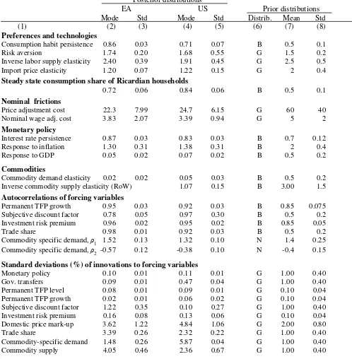
5. Estimation results
165.1. Posterior parameter estimates
The posterior estimates of key model parameters are reported in Table 1. (Estimates of other
parameters can be found in the Not-for-Publication Appendix.) The steady state consumption
share of the Ricardian household is estimated at 0.72 in the EA and 0.84 in the US. Estimated
consumption habit persistence is high in the EA (0.86) and the US (0.71), which indicates a
sluggish adjustment of consumption to income shocks. The estimated risk aversion coefficient is
1.74 in the EA and 1.68 in the US. The parameter estimates suggest a slightly lower labor supply
elasticity in the US than in the EA. Price elasticities of aggregate imports are 1.20 for the EA and
1.22 for the US.
The estimated substitution elasticity (in final good production) between commodities and
real domestic value added is 0.02 for the EA and 0.05 for the US (see row labelled ‘Commodity
demand elasticity’ in Table 1). That substitution elasticity corresponds to the price elasticity of
commodity demand. Our estimate of the price elasticity of RoW commodity supply is 0.55. Our low estimates of the EA and US price elasticities of commodity demand are in line with the
literature, but our estimate of the price elasticity of commodity supply is somewhat higher than
elasticities reported in the literature. See, e.g., Arezki et al. (2015) who report estimated price
elasticities of oil demand [supply] in the range of 0.02 [0.1].
15
We calibrate the substitution elasticity between energy and non-energy commodities at 0.5. The model estimation uses quarterly data on aggregate commodity imports of the EA and the US from RoW. Quarterly commodity import series disaggregated into energy vs. and non-energy are not available. Thus, the substitution elasticity between energy and non-energy commodities is not well identified—which is why that elasticity is calibrated.
16
15
The model estimates suggest substantial nominal price stickiness. Estimated price
adjustment cost parameters are slightly higher in the US (24.7) than in the EA (22.2), whereas
wage stickiness is higher in the EA (3.83) than in the US (3.39). The estimated shares of EA, US
and RoW manufactured goods exporters that set prices in destination-country currency (‘pricing
to market’, PTM) are 0.23, 0.16 and 0.53, respectively. Thus, PTM is markedly more prevalent
among RoW exporters.
Estimated monetary and fiscal policy parameters are similar across both regions. The
estimated EA and US interest rate rules indicate a strong response of the policy rate to domestic
inflation, and a weak response to domestic GDP.
The estimates also suggest that most exogenous variables are highly serially correlated.
The standard deviation of innovations to subjective discount factors, price mark-ups, trade shares,
commodity-specific demand and to commodity supply are sizable.
The model properties discussed in what follows are evaluated at the posterior mode of the
model parameters.
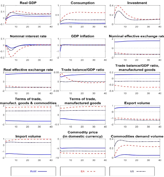
5.2. Impulse responses
This section discusses estimated dynamic effects of key shocks shown in Figs. 4a-4d. We
concentrate on the impact of supply and demand shocks originating in the RoW. The effects of
supply and demand shocks originating in the EA and the US on domestic GDP are qualitatively
similar to those predicted by standard DSGE models (see Kollmann et al. (2016) for a detailed
recent discussion), but in the setting here, those effects tend to be somewhat smaller because of
the endogenous response of commodity prices. In all impulse response plots, the responses of
RoW, EA and US variables are represented by continuous blue, dashed red and dash-dotted black
lines, respectively.
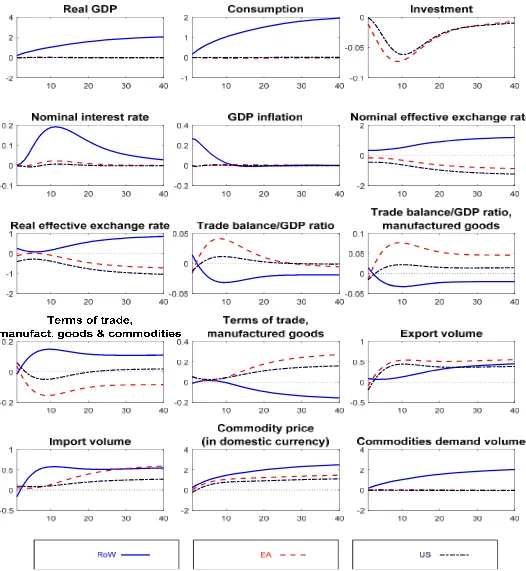
5.2.1. Effects of a persistent RoW TFP shock
Our model estimates suggest that persistent RoW TFP shocks were the main drivers of historical
RoW GDP fluctuations (see historical shock decomposition in Fig. 5b, discussed below). Fig. 4a
shows dynamic responses to a persistent positive shock to the RoW TFP growth rate that
permanently raises the level of RoW GDP by about 2% within 10 years. The persistent increase
in the supply of RoW tradables triggers a deterioration of the RoW terms of trade for
16
the same time, the expectation of a persistent rise in RoW TFP and GDP boosts RoW aggregate
demand. This explains why RoW inflation increases.
Because of adjustment frictions (consumption habits, credit frictions, investment
adjustment costs), the response of domestic and foreign absorption is nevertheless quite gradual.
This explains why the effect on trade balances is relatively modest, despite stronger responses of
gross trade flows.17 (All trade balance responses pertain to the nominal trade balance normalized by nominal GDP.) Initially, the Euro and Dollar appreciation dominates the response of EA and
US trade balances, which fall on impact; however, these trade balances quickly rise because of
higher RoW demand for EA and US export goods. US and EA export volumes stabilize rapidly at
higher levels, while import volumes grow more gradually.
Higher growth in RoW TFP raises commodity prices. This effect is strong enough to
induce a slight improvement of the overall RoW terms of trade. The rise in commodity prices
offsets the positive export demand effect on EA and US GDP. EA and US GDP are barely
affected by the positive shock to RoW TFP.
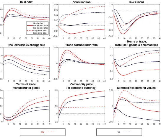
The role of the endogenous commodity price channel for international shock transmission
is highlighted in Fig. 4d, where we compare dynamic responses to the RoW TFP shock across the
baseline model (flexible commodity price) and a model variant in which the US dollar price of
commodities does not respond to the shock.18 The responses of EA and US real GDP are more
positive in the model variant with constant dollar commodity prices, but remain modest.19 In
other terms, the endogenous commodity price response in our baseline model dampens the
strength of the GDP spillover from RoW to the EA and the US.
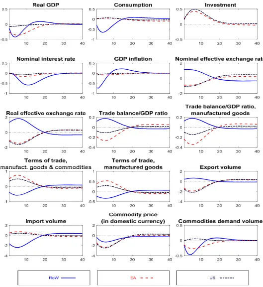
5.2.2. Effects of a RoW aggregate demand shock
Aggregate demand shocks in RoW too were key drivers of historical RoW GDP growth, and
these shocks also mattered significantly for historical EA and US trade balance fluctuations (see
shock decompositions in Figs. 5e and 5f, discussed below). Fig. 4b shows dynamic responses to a
negative aggregate demand shock in RoW, namely a persistent rise in the subjective discount
factor of RoW households (i.e. a positive saving shock). The shock reduces RoW GDP and RoW
17
By contrast, in a textbook permanent income model without adjustment frictions, persistent TFP growth rate shocks trigger rapid and strong responses of aggregate demand and, thus, of trade balances (Obstfeld and Rogoff (1996)).
18
In that model variant, the supply of commodities is assumed to be infinitely elastic, at the given dollar price (all remaining model parameters are unchanged). Considering a fixed dollar commodity price provides an interesting perspective on the role of commodity price dynamics, because of widespread dollar invoicing in global commodity markets.
19
17
import demand, and it depreciates the RoW currency. EA and US GDP fall, and EA and US trade
balances deteriorate. The adverse RoW aggregate demand shock markedly reduces commodity
prices, which weakens the negative international GDP spillover effect, compared to a model
variant with unresponsive dollar commodity prices. RoW aggregate demand shocks are thus
potential contributors to the high empirical volatility of commodity prices.
5.2.3. Effects of a RoW commodity supply shock
The previous discussion shows that commodity prices respond to aggregate supply and demand shocks. In addition, commodity prices exhibit strong responses to commodity supply shocks and
to commodity-specific demand shocks. The model estimates suggest that these shocks are highly
persistent.
Fig.4c. presents dynamic responses to a permanent positive commodity supply shock
(RoW). The shock triggers a permanent fall in commodity prices, and a strong nominal and real
depreciation of the RoW currency. It permanently raises GDP and absorption in the three regions.
The commodity supply shock triggers a strong rise in RoW gross export volumes, and a
contraction in RoW gross import volumes. Due to the low price elasticity of commodity demand,
a positive RoW commodity supply shock lowers the commodity export revenue received by
RoW, in domestic GDP units. Thus, the commodity trade balances of the EA and US (in GDP
units) improve. The sharp fall in commodity prices also explains why real consumption increases
much less in RoW than in the EA and the US. The RoW commodity supply shock improves the
EA and US terms of trade for manufactured goods, and it deteriorates the EA and US trade
balances for manufactures. Thus, the responses of the manufactures’ trade balance have an
off-setting (stabilizing) effect on the overall trade balance. At the estimated model parameters, the
response of the overall US trade balance is close to zero, while there is a noticeable improvement
in the overall EA trade balance.
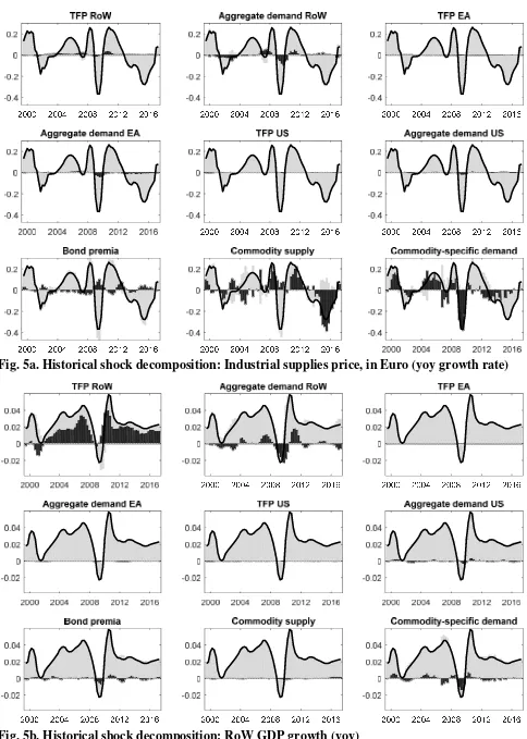
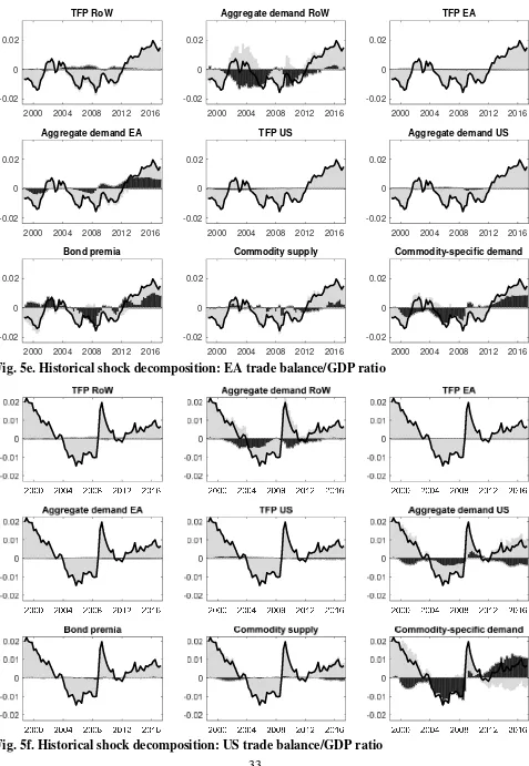
5.3. Historical shock decompositions
To quantify the role of different shocks as drivers of endogenous variables in the period
1999-2017, we plot the estimated contribution of these shocks to historical time series. Figs. 5a-5f
show historical shock decompositions of year-on-year (yoy) growth rates of the commodity price
(in Euro), and of RoW, EA and US GDP; also shown are historical shock decompositions of EA
and US trade balance/GDP ratios. In each sub-plot, the continuous thick black line shows
18
show the contribution of different groups of exogenous shocks (see below) to the historical data,
while stacked light bars show the contribution of the remaining shocks. Bars above the horizontal
axis represent positive shock contributions, while bars below the horizontal axis show negative
shock contributions.
Given the large number of shocks, we group together the contributions of related shocks.
Specifically, ‘TFP RoW’, ‘TFP EA’ and ‘TFP US’ represent the contributions of permanent and
transitory productivity shocks in RoW, the EA, and the US, respectively. ‘Aggregate demand
RoW’, ‘Aggregate demand EA’ and ‘Aggregate demand US’ capture the effect of aggregate
demand shocks (including household saving shocks, fiscal/monetary policy shocks and
investment risk premium shocks). ‘Bond premia’ shocks represent the contribution of shocks to
UIP conditions. ‘Commodity supply’ shocks represent shocks to RoW commodity supply.
‘Commodity-specific demand’ shocks represent the combined effect of EA and US
commodity-specific demand shocks (i.e. shocks to the commodity intensity of EA and US final good
production; see Sect. 3.2.2).20
5.3.1. Commodity (industrial supplies) prices
According to our estimates, historical commodity prices were mainly driven by EA and US
commodity-specific demand shocks, and by commodity supply shocks (see Fig. 5a).
Commodity-specific demand shocks were the major drivers of the pre-crisis commodity price boom, and of
the price collapse during the financial crisis, while commodity supply shocks were key drivers of
the post-crisis commodity price contraction.
Adverse aggregate demand shocks in the three regions made a smaller, but noticeable, contribution to the sharp commodity price contraction during the financial crisis. Aggregate
demand shocks had only a minor role for commodity prices, before and after the crisis.
Throughout the sample period, TFP shocks had a negligible effect on commodity prices.
To understand the central role of EA and US commodity-specific demand shocks for
historical commodity prices, according to the estimated model, one should note that the fitted
commodity-specific demand shocks account for fluctuations in commodity demand that are not
explained by movement in EA and US GDP and in the real commodity price (see Sect. 3.2.2).
Despite its richness, the model abstracts from some key real world drivers of EA and US
commodity demand. Thus, fitted commodity-specific demand shocks may capture the effect of a
20
19
range of empirical disturbances, besides pure shocks to the commodity intensity of EA and US
final good production.
Recall, in particular, that the model abstracts from US (and EA) commodity production
and exports. Yet, US crude oil production doubled between 2010 and 2015. Our estimated model
largely attributes the post-crisis fall in US net commodity imports to negative US
commodity-specific demand shocks. Those fitted shocks probably partly reflect the post-crisis expansion of
US commodity production.
The commodity-specific demand shocks identified by the model may also capture
changes in the sectoral composition of aggregate real activity that are not accounted for by our
theoretical production structure. During recessions, highly commodity-intensive sectors
(manufacturing) tend to reduce output much more strongly than less commodity-intensive sectors
(services). The model does not capture that cyclical composition effect. This may help to
understand why the model largely attributes the collapse in commodity prices during the Great
Financial Crisis to negative commodity-specific demand shocks.21 However, it seems implausible
that the post-crisis fall in commodity prices was mainly driven by adverse aggregate
demand/supply shocks, as by 2013 GDP growth had resumed both in the US and the EA, after
having recovered earlier in the RoW. This implies that ‘commodity-specific’ supply and demand
factors are the most likely drivers of the post-crisis dynamics of commodity prices and
commodity imports.
Empirically, EA and US commodity demand is procyclical, and much more volatile than
GDP; the fitted commodity-specific demand shocks too are procyclical and highly volatile.22 In
an attempt to capture effects of aggregate real activity on commodity demand that are potentially
missing from the baseline model, we have experimented with a model variant that features a
direct impact of aggregate activity on the EA and US commodity-specific demand shifters ( ;stis
see Sect. 3.2.2). Specifically, those demand shifters are assumed to be (increasing) functions of
21
Forni et al. (2015), who estimated a two-country (EA, RoW) DSGE model with oil, too find a non-negligible role of commodity-specific demand shocks for the oil price, but in their set-up aggregate demand shocks matter significantly for the oil price. Forni et al. (2015) do not use data on regional oil demand/imports. By contrast, our estimation uses data on EA and US commodity net imports from RoW, as well as data on the determinants of commodity demand (real GDP, relative commodity price), which allows a direct identification of commodity-specific demand shocks, in the context of our model.
22
20
domestic capacity utilization, and of exogenous region-specific disturbances.23 The slope
coefficients are set by regressing fitted EA and US commodity-specific demand shocks, from our
baseline model, on historical EA and US capacity utilization data. Note that this experiment is set
up to maximize the influence of a highly cyclical variable (capacity utilization) on commodity
demand. In this experiment, the exogenous shocks to the EA and US commodity-specific demand
shifter still explain about half of the commodity price collapse during the Global Financial Crisis.
Overall, during our sample period (1999-2017), the influence of exogenous commodity-specific
demand shocks on commodity prices shrinks by about one third, while the impact of aggregate
demand shocks rises slightly. However, most importantly, exogenous commodity supply shocks
and exogenous commodity-specific demand shocks remain the main drivers of commodity prices,
especially during the crisis period, and they continue to be significant drivers of the
post-crisis trade balance reversal in the EA and US (see below)
5.3.2. RoW GDP growth
According to the estimated model, strong RoW GDP growth was mainly driven by persistent
positive domestic TFP shocks (see Fig. 5b). The growth of RoW TFP and GDP was, however,
interrupted in 2001 and 2008-9, i.e. by the recessions following the dot-com bubble and by the
Global Financial Crisis. After 2010, we again detect sustained positive TFP contributions to RoW
GDP growth. Domestic aggregate demand shocks too were influential drivers of RoW GDP
fluctuations. The model identifies negative RoW aggregate demand shocks in the late 1990s and
early 2000s that reflected increased RoW household saving rates (perhaps due to heightened risk
aversion in the aftermath of the Asian debt crisis). RoW aggregate demand remained weak until
the mid-2000s. A large negative RoW aggregate demand shock occurred during the Global
Financial Crisis, which was followed by positive RoW aggregate demand shocks in 2010-11.
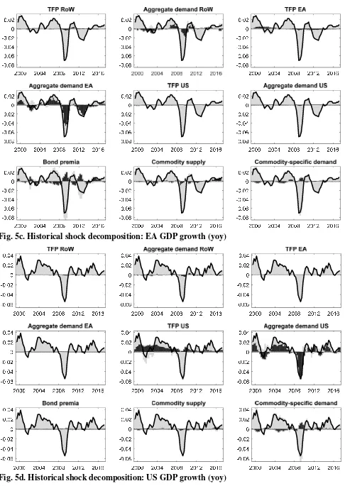
5.3.3. EA and US GDP growth
Fluctuations in EA and US GDP growth were largely driven by domestic aggregate demand
shocks (in particular by household saving shocks and by investment shocks); see Figs. 5c and 5d.
After the Global Financial Crisis, domestic aggregate demand and GDP rebounded more quickly
in the US than in the EA, which experienced a recession in 2012-13. In both the US and the EA,
monetary and fiscal policy provided some GDP stabilization (not shown in Figures). The
23
0 1 ,
is
t t t
21
contribution of domestic TFP shocks to historical GDP fluctuations has been much smaller in the
EA and US than in RoW. Consistent with the weak international transmission effects discussed
above, we find that EA and US GDP were hardly affected by RoW TFP shocks. However, RoW
aggregate demand shocks had noticeable positive spillover effects on EA GDP.
5.3.4. EA and US trade balances
In the period before the financial crisis, the US trade balance declined markedly, while the EA
trade balance was trendless and fluctuated around zero; after the crisis, the EA and US trade
balances both rose strongly and persistently (see discussion in Sect. 2).
Our model estimates show that positive shocks to RoW saving and to US aggregate
demand had a negative influence on the US trade balance, during the pre-crisis period (see Fig.
5f). Before the crisis, adverse RoW aggregate demand shocks and positive EA aggregate demand
shocks also affected the EA trade balance negatively (Fig. 5e); however, we identify
countervailing forces on the EA trade balance, in particular the depreciation of the Euro in the
early 2000s.24 Note that our estimates are consistent with a RoW ‘saving glut’ effect (Bernanke
(2005) on both US and EA trade balances.
In 2002-08, positive commodity-specific demand shocks had a significant negative
influence on both the EA and US trade balance; however, these shocks were probably partly
induced by the pre-crisis boom itself (strong cyclical responsiveness of net commodity imports).
Our estimation results suggest that commodity shocks played a central role for the
post-crisis EA and US trade balance reversals. In the US, large negative commodity-specific demand
shocks (that likely in part reflect the expansion of US commodity production; see discussion
above) had an especially strong and sustained positive influence on net exports, after the crisis. In
the EA, too, negative commodity-specific demand shocks contributed markedly to the post-crisis
trade balance increase (positive commodity supply shocks likewise contributed to the EA trade balance reversal).
However, the persistent post-crisis weakness of EA aggregate demand and the
depreciation of the Euro also played a significant part in the rise of the EA trade balance. Strong
RoW aggregate demand during the post-crisis period too contributed to the EA and US trade
balance improvements. The more rapid and stronger post-crisis rebound of US domestic
aggregate demand actually had a negative influence on the US trade balance.
24
22
6. Conclusion
This paper identifies key shocks that have driven economic fluctuations and external adjustment,
in the Euro Area (EA), the US and the rest of the world (RoW), since 1999. Our empirical
analysis is based on an estimated three region DSGE model of the world economy that includes a
commodity sector. The sample period saw very large commodity price fluctuations. We find that
RoW GDP growth was largely driven by persistent TFP shocks, while EA and US GDP
fluctuations mainly reflected domestic aggregate demand shocks. The paper highlights the key
contribution of commodity shocks for the dynamics of EA and US trade balances, particularly for
the strong and persistent post-crisis EA and US trade balance improvements. Aggregate demand
shocks originating in RoW too had a significant impact on EA and US trade balances. The
broader lesson of this paper is thus that Emerging Markets (RoW) and commodity shocks are
23
References
Adjemian, Stéphane, Houtan Bastani, Michel Juillard, Frédéric Karamé, Ferhat Mihoubi, George Perendia, Johannes Pfeifer, Marco Ratto and Sébastien Villemot, 2011. Dynare: Reference Manual, Version 4. Dynare Working Papers, 1, CEPREMAP.
Arezki, Rabah, Zoltan Jakab, Douglas Laxton, Akito Matsumoto, Armen Nurbekyan, Hou Wang, and Jiaxiong Yao, 2017. Oil Prices and the Global Economy. IMF Working Paper WP/17/15. Backus, David and Mario Crucini, 2000. Oil Prices and the Terms of Trade. Journal of
International Economics 50, 185–213.
Baffes, John, Ayhan Kose, Franziska Ohnsorge and Marc Stocke, 2015. The Great Plunge in Oil Prices: Causes, Consequence and Policy Responses. World Bank Policy Research Note.
Bernanke, Ben, 2005. Sandridge Lecture, Virginia Association of Economists.
Betts, Caroline and Michael B. Devereux, 2000. Exchange rate dynamics in a model of pricing-to-market. Journal of International Economics 50, 215–244.
Bornstein, Gideon, Per Krusell and Sergio Rebelo, 2018. Lags, Costs, and Stocks: An Equilibrium Model of the Oil Industry. Working Paper, Northwestern University.
Caldara, Dario, Michele Cavallo and Matteo Iacoviello, 2017. Oil Price Elasticities and Oil Price Fluctuations. Working Paper, Federal Reserve Board.
Dieppe, Alastair, Georgios Georgiadis, Martino Ricci, Ine Van Robays and Björn van Roye, 2018. ECB-Global: Introducing the ECB’s Global Macroeconomic Model for Spillover analysis. Economic Modelling 72, 78-98.
European Central Bank, 2010. Energy Markets and the European Macroeconomy. ECB Occasional Paper 113.
Finn, Mary, 1995. Variance Properties of Solow’s Productivity Residual and Their Cyclical Implications. Journal of Economic Dynamics & Control 19, 1249-1281.
Finn, Mary, 2000. Perfect Competition and the Effects of Energy Price Increases on Economic Activity. Journal of Money, Credit and Banking 32, 400-416.
Forni, Lorenzo, Andrea Gerali, Alessandro Notarpietro and Massimiliano Pisani, 2015. Euro Area, Oil and Global Shocks: An Empirical Model-Based Analysis. Journal of Macroeconomics 46, 295-314.
Gars, Johan and Conny Olovsson, 2017. International Business Cycles: Quantifying the Effects of a World Market for Oil. Working Paper, Riksbank (Sweden).
in’t Veld, Jan, Robert Kollmann, Beatrice Pataracchia, Marco Ratto and Werner Roeger, 2014. International Capital Flows and the Boom-Bust Cycle in Spain. Journal of International Money and Finance 48, 314-335.
Jacks, David, 2013. From Boom to Bust: A Typology of Real Commodity Prices in the Long Run. NBER Working Paper 18874.
Jacks, David, 2016. Chartbook for “From Boom to Bust”, Working Paper, Simon Fraser University.
Kilian, Lutz, Alessandro Rebucci and Nikola Spatafora, 2009. Oil shocks and external balances. Journal of International Economics 77, 181-194.
Kilian, Lutz and Bruce Hicks, 2012. Did Unexpectedly Strong Economic Growth Cause the Oil Price Shock of 2003-2008? Journal of Forecasting.
Kollmann, Robert, 2002. Monetary Policy Rules in the Open Economy: Effects on Welfare and Business Cycles. Journal of Monetary Economics 49, 989-1015.
Kollmann, Robert, 2004. Welfare Effects of a Monetary Union: the Role of Trade Openness. Journal of the European Economic Association 2, 289-301.
24
Kollmann, Robert, Beatrice Pataracchia, Marco Ratto, Werner Roeger and Lukas Vogel, 2016. The Post-Crisis Slump in the Euro Area and the US: Evidence from an Estimated Three-Region DSGE Model. European Economic Review 88, 21–41.
McKibbin, Warwick and Jeffery Sachs, 1991. Global Linkages. The Brookings Institution.
McKibbin, Warwick and Andrew Stoeckel, 2018. Modelling a Complex World: Improving Macro-Models. Oxford Review of Economic Policy 34, 329–347.
Miura, Shogo, 2017. World Price Shocks and Business Cycles. Working Paper, Université Libre de Bruxelles.
Obstfeld, Maurice and Kenneth Rogoff, 1996. Foundations of International Macroeconomics. MIT Press.
Peersman, Gert and Ine Van Robays, 2009. Oil and the European Economy. Economic Policy. Ratto Marco, Werner Roeger and Jan in ’t Veld, 2009. QUEST III: An Estimated Open-Economy
DSGE Model of the Euro Area with Fiscal and Monetary Policy, Economic Modelling, 26, 222–33.
25
Fig. 1a. Growth rate of real GDP (year-on-year, in %)
Fig. 1b. Shares in World nominal GDP (in US dollars, based on nom. exch.rates)
Fig. 2a. Commodity prices (in dollars, 2009=100)
26
Fig. 3a.EA Net exports by product (in%EA GDP)
Note: these series are only available for 2003- (annual). Fig.3b.EA Net exports by region (in % EA GDP)
27
Fig. 4a Dynamic effects of positive shock to trend growth rate of RoW TFP (1 standard deviation)
28
Fig. 4b. Dynamic effects of negative aggregate demand shock in RoW (1 standard deviation)
29
Fig. 4c. Dynamic effects of positive shock to RoW commodity supply (1 standard deviation)
30 5 10 15 20 25 30 35 40
-0.1 -0.05 0 0.05 Real GDP Steady state Endogenous price Endogenous price Exogenous price Exogenous price
5 10 15 20 25 30 35 40 -0.04 -0.02 0 0.02 0.04 0.06 0.08 Consumption
5 10 15 20 25 30 35 40 -0.08 -0.06 -0.04 -0.02 0 0.02 Investment
5 10 15 20 25 30 35 40 -1.5
-1 -0.5 0
0.5 Real effective exchange rate
5 10 15 20 25 30 35 40 -0.05
0
0.05 Trade balance/GDP ratio
5 10 15 20 25 30 35 40 -0.2
-0.1 0 0.1 0.2
Terms of trade,
manufact. goods & commodities
5 10 15 20 25 30 35 40 0
0.1 0.2 0.3 0.4
Terms of trade, manufactured goods
5 10 15 20 25 30 35 40 -0.5 0 0.5 1 1.5 Commodity price (in domestic currency)
5 10 15 20 25 30 35 40 -0.05
0
0.05 Commodities demand volume
[image:31.612.51.596.62.526.2]EA US
Fig. 4d. Dynamic effects of a positive shock to trend growth rate of RoW TFP (1 standard deviation) on EA and US variables: comparison of baseline model (flexible commodity prices) vs. model version with fixed commodity prices (in dollars)
31
Fig. 5a. Historical shock decomposition: Industrial supplies price, in Euro (yoy growth rate)
32
Fig. 5c. Historical shock decomposition: EA GDP growth (yoy)
33
TFP RoW
2000 2004 2008 2012 2016
-0.02 0 0.02
Aggregate demand RoW
2000 2004 2008 2012 2016
-0.02 0 0.02
TFP EA
2000 2004 2008 2012 2016
-0.02 0 0.02
Aggregate demand EA
2000 2004 2008 2012 2016
-0.02 0 0.02
TFP US
2000 2004 2008 2012 2016
-0.02 0 0.02
Aggregate demand US
2000 2004 2008 2012 2016
-0.02 0 0.02
Bond premia
2000 2004 2008 2012 2016
-0.02 0 0.02
Commodity supply
2000 2004 2008 2012 2016
-0.02 0 0.02
Commodity-specific demand
2000 2004 2008 2012 2016
[image:34.612.76.553.45.736.2]-0.02 0 0.02
[image:34.612.78.557.50.388.2]Fig. 5e. Historical shock decomposition: EA trade balance/GDP ratio
34
Table 1. Prior and posterior distributions of key estimated model parameters
Posterior distributions
EA US Prior distributions
Mode Std Mode Std Distrib. Mean Std
(1) (2) (3) (4) (5) (6) (7) (8)
Preferences and technologies
Consumption habit persistence 0.86 0.03 0.71 0.07 B 0.5 0.1 Risk aversion 1.74 0.20 1.68 0.55 G 1.5 0.2 Inverse labor supply elasticity 2.40 0.39 1.91 0.45 G 2.5 0.5 Import price elasticity 1.20 0.07 1.22 0.15 G 2 0.4
Steady state consumption share of Ricardian households
0.72 0.06 0.84 0.06 B 0.5 0.1
Nominal frictions
Price adjustment cost 22.3 7.99 24.7 6.15 G 60 40 Nominal wage adj. cost 3.83 2.07 3.39 0.94 G 5 2
Monetary policy
Interest rate persistence 0.87 0.03 0.83 0.03 B 0.7 0.12 Response to inflation 1.30 0.31 1.38 0.31 B 2 0.4 Response to GDP 0.05 0.02 0.07 0.02 B 0.5 0.2
Commodities
Commodity demand elasticity 0.02 0.02 0.05 0.03 B 0.5 0.2 Inverse commodity supply elasticity (RoW) 1.07 0.15 B 3.00 1.5
Autocorrelations of forcing variables
Permanent TFP growth 0.95 0.03 0.92 0.03 B 0.85 0.075 Subjective discount factor 0.78 0.05 0.97 0.30 B 0.5 0.2 Investment risk premium 0.96 0.02 0.95 0.02 B 0.85 0.05 Trade share 0.98 0.01 0.92 0.03 B 0.5 0.2 Commodity specific demand, ρ1 1.52 0.13 1.32 0.10 N 1.4 0.25 Commodity specific demand, ρ2 -0.57 0.12 -0.38 0.10 N -0.4 0.15
Standard deviations (%) of innovations to forcing variables