Learning Word Representations by Jointly Modeling Syntagmatic and Paradigmatic Relations

Learning Word Representations by Jointly Modeling

Syntagmatic and Paradigmatic Relations

Fei Sun, Jiafeng Guo, Yanyan Lan, Jun Xu,

and

Xueqi Cheng

CAS Key Lab of Network Data Science and Technology

Institute of Computing Technology

Chinese Academy of Sciences, China

[email protected]

{guojiafeng,lanyanyan,junxu,cxq}@ict.ac.cn

Abstract

Vector space representation of words has been widely used to capture fine-grained linguistic regularities, and proven to be successful in various natural language pro-cessing tasks in recent years. However, existing models for learning word repre-sentations focus on either syntagmatic or paradigmatic relations alone. In this pa-per, we argue that it is beneficial to jointly modeling both relations so that we can not only encode different types of linguistic properties in a unified way, but also boost the representation learning due to the mu-tual enhancement between these two types of relations. We propose two novel dis-tributional models for word representation using both syntagmatic and paradigmatic relations via a joint training objective. The proposed models are trained on a public Wikipedia corpus, and the learned rep-resentations are evaluated on word anal-ogy and word similarity tasks. The re-sults demonstrate that the proposed mod-els can perform significantly better than all the state-of-the-art baseline methods on both tasks.

1 Introduction

Vector space models of language represent each word with a real-valued vector that captures both semantic and syntactic information of the word. The representations can be used as basic features in a variety of applications, such as information re-trieval (Manning et al., 2008), named entity recog-nition (Collobert et al., 2011), question answer-ing (Tellex et al., 2003), disambiguation (Sch¨utze, 1998), and parsing (Socher et al., 2011).

A common paradigm for acquiring such repre-sentations is based on thedistributional hypothe-sis (Harris, 1954; Firth, 1957), which states that

is wolf

The a fierce animal.

is tiger

The a fierce animal.

syntagmatic

syntagmatic paradigmatic

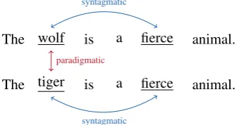
Figure 1: Example for syntagmatic and paradig-matic relations.

words occurring in similar contexts tend to have similar meanings. Based on this hypothesis, vari-ous models on learning word representations have been proposed during the last two decades.

According to the leveraged distributional infor-mation, existing models can be grouped into two categories (Sahlgren, 2008). The first category mainly concerns thesyntagmatic relationsamong the words, which relate the words that co-occur in the same text region. For example, “wolf” is close to “fierce” since they often co-occur in a sen-tence, as shown in Figure 1. This type of models learn the distributional representations of words based on the text region that the words occur in, as exemplified by Latent Semantic Analysis (LSA) model (Deerwester et al., 1990) and Non-negative Matrix Factorization (NMF) model (Lee and Se-ung, 1999). The second category mainly cap-tures paradigmatic relations, which relate words that occur with similar contexts but may not co-occur in the text. For example, “wolf” is close to “tiger” since they often have similar context words. This type of models learn the word rep-resentations based on the surrounding words, as exemplified by the Hyperspace Analogue to Lan-guage (HAL) model (Lund et al., 1995), Con-tinuous Bag-of-Words (CBOW) model and Skip-Gram (SG) model (Mikolov et al., 2013a).

take both syntagmatic and paradigmatic relations into account to build a good distributional model. Firstly, in distributional meaning acquisition, it is expected that a good representation should be able to encode a bunch of linguistic properties. For example, it can put semantically related words close (e.g., “microsoft” and “office”), and also be able to capture syntactic regularities like “big is to bigger as deep is to deeper”. Obviously, these linguistic properties are related to both syntag-matic and paradigsyntag-matic relations, and cannot be well modeled by either alone. Secondly, syntag-matic and paradigsyntag-matic relations are complimen-tary rather than conflicted in representation learn-ing. That is relating the words that co-occur within the same text region (e.g., “wolf” and “fierce” as well as “tiger” and “fierce”) can better relate words that occur with similar contexts (e.g., “wolf” and “tiger”), and vice versa.

Based on the above analysis, we propose two new distributional models for word representa-tion using both syntagmatic and paradigmatic re-lations. Specifically, we learn the distributional representations of words based on the text region (i.e., the document) that the words occur in as well as the surrounding words (i.e., word sequences within some window size). By combining these two types of relations either in a parallel or a hier-archical way, we obtain two different joint training objectives for word representation learning. We evaluate our new models in two tasks, i.e., word analogy and word similarity. The experimental results demonstrate that the proposed models can perform significantly better than all of the state-of-the-art baseline methods in both of the tasks.

2 Related Work

The distributional hypothesis has provided the foundation for a class of statistical methods for word representation learning. According to the leveraged distributional information, existing models can be grouped into two categories, i.e., syntagmatic models and paradigmatic models.

Syntagmatic modelsconcern combinatorial re-lations between words (i.e., syntagmatic rela-tions), which relate words that co-occur within the same text region (e.g., sentence, paragraph or doc-ument).

For example, sentences have been used as the text region to acquire co-occurrence information by (Rubenstein and Goodenough, 1965; Miller

and Charles, 1991). However, as pointed our by Picard (1999), the smaller the context regions are that we use to collect syntagmatic information, the worse the sparse-data problem will be for the resulting representation. Therefore, syntagmatic models tend to favor the use of larger text regions as context. Specifically, a document is often taken as a natural context of a word following the liter-ature of information retrieval. In these methods, a words-by-documents co-occurrence matrix is built to collect the distributional information, where the entry indicates the (normalized) frequency of a word in a document. A low-rank decomposition is then conducted to learn the distributional word representations. For example, LSA (Deerwester et al., 1990) employs singular value decomposition by assuming the decomposed matrices to be or-thogonal. In (Lee and Seung, 1999), non-negative matrix factorization is conducted over the words-by-documents matrix to learn the word represen-tations.

Paradigmatic models concern substitutional relations between words (i.e., paradigmatic rela-tions), which relate words that occur in the same context but may not at the same time. Unlike syntagmatic model, paradigmatic models typically collect distributional information in a words-by-words co-occurrence matrix, where entries indi-cate how many times words occur together within a context window of some size.

the Global Vectors (GloVe) for word representa-tion.

Alternatively, neural probabilistic language models (NPLMs) (Bengio et al., 2003) learn word representations by predicting the next word given previously seen words. Unfortunately, the training of NPLMs is quite time consuming, since com-puting probabilities in such model requires nor-malizing over the entire vocabulary. Recently, Mnih and Teh (2012) applied Noise Contrastive Estimation (NCE) to approximately maximize the probability of the softmax in NPLM. Mikolov et al. (2013a) further proposed continuous bag-of-words (CBOW) and skip-gram (SG) models, which use a simple single-layer architecture based on inner product between two word vectors. Both models can be learned efficiently via a simple vari-ant of Noise Contrastive Estimation,i.e., Negative sampling (NS) (Mikolov et al., 2013b).

3 Our Models

In this paper, we argue that it is important to jointly model both syntagmatic and paradigmatic rela-tions to learn good word representarela-tions. In this way, we not only encode different types of linguis-tic properties in a unified way, but also boost the representation learning due to the mutual enhance-ment between these two types of relations.

We propose two joint models that learn the dis-tributional representations of words based on both the text region that the words occur in (i.e., syntag-matic relations) and the surrounding words (i.e., paradigmatic relations). To model syntagmatic re-lations, we follow the previous work (Deerwester et al., 1990; Lee and Seung, 1999) to take docu-ment as a nature text region of a word. To model paradigmatic relations, we are inspired by the re-cent work from Mikolov et al. (Mikolov et al., 2013a; Mikolov et al., 2013b), where simple mod-els over word sequences are introduced for effi-cient and effective word representation learning.

In the following, we introduce the notations used in this paper, followed by detailed model de-scriptions, ending with some discussions of the proposed models.

3.1 Notation

Before presenting our models, we first list the no-tations used in this paper. Let D={d1, . . . , dN} denote a corpus of N documents over the word vocabulary W. The contexts for word

sat

. . . the cat

sat on the. . .

cat

on

the the

cn i−1

cn i+1

cn i+2

cn i−2

dn

wn i ...

...

Projection

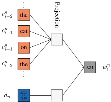
Figure 2: The framework for PDC model. Four words (“the”, “cat”, “on” and “the”) are used to predict the center word (“sat”). Besides, the doc-ument in which the word sequence occurs is also used to predict the center word (“sat”).

wn

i∈W (i.e. i-th word in document dn) are the words surrounding it in an L-sized window (cn

i−L, . . . , cni−1, cni+1, . . . , cni+L)∈H, wherecnj ∈

W, j∈{i−L, . . . , i−1, i+1, . . . , i+L}. Each doc-umentd ∈ D, each wordw ∈ W and each con-textc ∈ W is associated with a vector ⃗d∈ RK_,

⃗w ∈ RK _{and⃗c ∈ R}K_{, respectively, whereK is} the embedding dimensionality. The entries in the vectors are treated as parameters to be learned.

3.2 Parallel Document Context Model

The first proposed model architecture is shown in Figure 2. In this model, a target word is predicted by its surrounding context, as well as the docu-ment it occurs in. The former prediction task cap-tures the paradigmatic relations, since words with similar context will tend to have similar represen-tations. While the latter prediction task models the syntagmatic relations, since words co-occur in the same document will tend to have similar represen-tations. More detailed analysis on this will be pre-sented in Section 3.4. The model can be viewed as an extension of CBOW model (Mikolov et al., 2013a), by adding an extra document branch. Since both the context and document are parallel in predicting the target word, we call this model the Parallel Document Context (PDC) model.

model is the log likelihood of all words

ℓ=∑N n=1

∑

wn i∈dn

(

logp(wn

i|hni)+ logp(wni|dn))

wherehn

i denotes the projection ofwni’s contexts, defined as

hn_i =f(cn_i−L, . . . , c_in₋₁, cn_i+1, . . . , cn_i+L)

where f(·) can be sum, average, concatenate or max pooling of context vectors1_{. In this paper, we}

use average, as that ofword2vectool.

We use softmax function to define the probabil-itiesp(wn

i|hni)andp(wni|dn)as follows:

p(win|hni) = exp(

⃗ wn

i ·h⃗ni) ∑

w∈Wexp(⃗w·h⃗ni)

(1)

p(wn

i|dn) = exp(w⃗ n i ·d⃗n) ∑

w∈Wexp(⃗w·d⃗n) (2)

where h⃗n

i denotes projected vector ofwni’s con-texts.

To learn the model, we adopt the negative sam-pling technique (Mikolov et al., 2013b) for effi-cient learning since the original objective is in-tractable for direct optimization. The negative sampling actually defines an alternate training ob-jective function as follows

ℓ= N ∑

n=1

∑

wn i∈dn

(

logσ(w⃗n

i·h⃗ni)+ logσ(w⃗in·d⃗n)

+k·Ew′_∼Pnwlogσ(w⃗′·h⃗n_i)

+k·Ew′_∼Pnwlogσ(w⃗′·d⃗_n))

(3)

whereσ(x) = 1/(1 + exp(−x)), k is the num-ber of “negative” samples,w′_{denotes the sampled}

word, andPnwdenotes the distribution of negative

word samples. We use stochastic gradient descent (SGD) for optimization, and the gradient is calcu-lated via back-propagation algorithm.

3.3 Hierarchical Document Context Model

Since the above PDC model can be viewed as an extension of CBOW model, it is natural to in-troduce the same document-word prediction layer into the SG model. This becomes our second

1_{Note that the context window sizeLcan be a function of}

the target wordwn

i. In this paper, we use the same strategy

asword2vectools which uniformly samples from the set

{1,2,· · ·, L}.

. . . the cat

sat on the. . .

sat

cat on the

the

dn

cn

i−1 cni+1 cni+2

cn i−2

· · · ·

Projection Projection

wn i

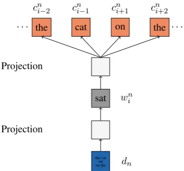
Figure 3: The framework for HDC model. The document is used to predict the target word (“sat”). Then, the word (“sat”) is used to predict the sur-rounding words (“the”, “cat”, “on” and “the”).

model architecture as shown in Figure 3. Specif-ically, the document is used to predict a target word, and the target word is further used to dict its surrounding context words. Since the pre-diction is conducted in a hierarchical manner, we name this model the Hierarchical Document Con-text (HDC) model. Similar as the PDC model, the syntagmatic relation in HDC is modeled by the document-word prediction layer and the word-context prediction layer models the paradigmatic relation.

Formally, the objective function of HDC model is the log likelihood of all words:

ℓ= N ∑

n=1

∑

wn i∈dn

( i_∑+L

j=i−L j̸=i

logp(cn_j|w_in)+ logp(w_in|dn) )

where p(wn

i|dn)is defined the same as in Equa-tion (2), andp(cn

j|wni)is also defined by a softmax function as follows:

p(cn_j|wn_i) = ∑exp(⃗cnj ·w⃗ni) c∈W exp(⃗c·w⃗ni)

training objective function

ℓ=∑N n=1

∑

wn i∈dn

( _∑i+L

j=i−L j̸=i

(

logσ(⃗cn j ·w⃗in)

+k·Ec′_∼Pnclogσ(⃗c′·w⃗n_i)

)

+ logσ(w⃗n

i·d⃗n) +k·Ew′_∼Pnwlogσ(w⃗′·d⃗_n)

)

wherekis the number of the negative samples,c′

andw′_{denotes the sampled context and word}

re-spectively, andPnc andPnw denotes the

distribu-tion of negative context and word samples respec-tively2_{. We also employ SGD for optimization,}

and calculate the gradient via back-propagation al-gorithm.

3.4 Discussions

In this section we first show how PDC and HDC models capture the syntagmatic and paradigmatic relations from the viewpoint of matrix factoriza-tion. We then talk about the relationship of our models with previous work.

As pointed out in (Sahlgren, 2008), to capture syntagmatic relations, the implementational basis is to collect text data in a words-by-documents co-occurrence matrix in which the entry indicates the (normalized) frequency of occurrence of a word in a document (or, some other type of text region, e.g., a sentence). While the implementational ba-sis for paradigmatic relations is to collect text data in a words-by-words co-occurrence matrix that is populated by counting how many times words oc-cur together within the context window. We now take the proposed PDC model as an example to show how it achieves these goals, and similar re-sults can be shown for HDC model.

The objective function of PDC with negative sampling in Equation (3) can be decomposed into the following two parts:

ℓ1=

∑

w∈W ∑

h∈H (

#(w, h)·logσ(⃗w·⃗h)

+k·#(h)·pnw(w)logσ(−⃗w·⃗h))

(4)

ℓ2=

∑

d∈D ∑

w∈W (

#(w, d)·logσ(⃗w·⃗d)

+k·|d|·pnw(w)logσ(−⃗w·⃗d))

(5)

where#(·,·)denotes the number of times the pair (·,·) appears in D, #(h)=∑_w∈W#(w, h), |d|

2_{Pncis not necessary to be the same asPnw.}

denotes the length of document d, the objective functionℓ1 corresponds to the context-word

pre-diction task andℓ2 corresponds to the

document-word prediction task.

Following the idea introduced by (Levy and Goldberg, 2014a), it is easy to show that the so-lution of the objective functionℓ1follows that

⃗w·⃗h= log( #(w, h)

#(h)·pnw(w))−logk

and the solution of the objective function ℓ2

fol-lows that

⃗w· ⃗d= log( #(w, d)

|d| ·pnw(w))−logk

It reveals that the PDC model with negative sam-pling is actually factorizing both a contexts co-occurrence matrix and a words-by-documents co-occurrence matrix simultaneously. In this way, we can see that the implementational basis of the PDC model is consistent with that of syntagmatic and paradigmatic models. In other words, PDC can indeed capture both syntagmatic and paradigmatic relations by processing the right distributional information. Please notice that the PDC model is not equivalent to direct combina-tion of existing matrix factorizacombina-tion methods, due to the fact that the matrix entries defined in PDC model are more complicated than the simple co-occurrence frequency (Lee and Seung, 1999).

When considering existing models, one may connect our models to the Distributed Memory model of Paragraph Vectors (PV-DM) and the Dis-tributed Bag of Words version of Paragraph Vec-tors (PV-DBOW) (Le and Mikolov, 2014). How-ever, both of them are quite different from our models. In PV-DM, the paragraph vector and con-text vectors are averaged or concatenated to pre-dict the next word. Therefore, the objective func-tion of PV-DM can no longer decomposed as the PDC model as shown in Equation (4) and (5). In other words, although PV-DM leverages both paragraph and context information, it is unclear how these information is collected and used in this model. As for PV-DBOW, it simply lever-ages paragraph vector to predict words in the para-graph. It is easy to show that it only uses the words-by-documents co-occurrence matrix, and thus only captures syntagmatic relations.

short) (Huang et al., 2012). The model defines two scoring components that contribute to the fi-nal score of a (word sequence, document) pair. The architecture of GCANLM seems similar to our PDC model, but exhibits lots of differences as follows: (1) GCANLM employs neural net-works as components while PDC resorts to simple model structure without non-linear hidden layers; (2) GCANLM uses weighted average of all word vectors to represent the document, which turns out to model words-by-words co-occurrence (i.e., paradigmatic relations) again rather than words-by-documents co-occurrence (i.e., syntagmatic re-lations); (3) GCANLM is a language model which predicts the next word given the preceding words, while PDC model leverages both preceding and succeeding contexts for prediction.

4 Experiments

In this section, we first describe our experimen-tal settings including the corpus, hyper-parameter selections, and baseline methods. Then we com-pare our models with baseline methods on two tasks,i.e., word analogy and word similarity. Af-ter that, we conduct some case studies to show that our model can better capture both syntagmatic and paradigmatic relations and how it improves the performances on semantic tasks.

4.1 Experimental Settings

We select Wikipedia, the largest online knowl-edge base, to train our models. We adopt the publicly available April 2010 dump3_{(Shaoul and}

Westbury, 2010), which is also used by (Huang et al., 2012; Luong et al., 2013; Neelakantan et al., 2014). The corpus in total has3,035,070articles and about1billion tokens. In preprocessing, we lowercase the corpus, remove pure digit words and non-English characters4_.

Following the practice in (Pennington et al., 2014), we set context window size as10and use 10negative samples. The noise distributions for context and words are set as the same as used in (Mikolov et al., 2013a), pnw(w) ∝ #(w)0.75.

We also adopt the same linear learning rate strat-egy described in (Mikolov et al., 2013a), where the initial learning rate of PDC model is 0.05, and

3_{http://www.psych.ualberta.ca/∼westburylab/downloads/}

westburylab.wikicorp.download.html

4_{We ignore the words less than 20 occurrences during}

training.

Table 1: Corpora used in baseline models.

model corpus size

C&W Wikipedia 2007 + Reuters RCV1 0.85B

HPCA Wikipedia 2012 1.6B

GloVe Wikipedia 2014+ Gigaword5 6B

GCANLM, CBOW, SG _{Wikipedia 2010 1B}

PV-DBOW, PV-DM

HDC is 0.025. No additional regularization is used in our models5_.

We compare our models with various state-of-the-art models including C&W (Collobert et al., 2011), GCANLM (Huang et al., 2012), CBOW, SG (Mikolov et al., 2013a), GloVe (Pennington et al., 2014), PV-DM, PV-DBOW (Le and Mikolov, 2014) and HPCA (Lebret and Collobert, 2014). For C&W, GCANLM6_{, GloVe and HPCA, we use}

the word embeddings they provided. For CBOW and SG model, we reimplement these two mod-els since the originalword2vectool uses SGD butcannotshuffle the data. Besides, we also im-plement PV-DM and PV-DBOW models due to (Le and Mikolov, 2014) has not released source codes. We train these four models on the same dataset with the same hyper-parameter settings as our models for fair comparison. The statistics of the corpora used in baseline models are shown in Table 1. Moreover, since different papers re-port different dimensionality, to be fair, we con-duct evaluations on three dimensions (i.e., 50, 100, 300) to cover the publicly available results7_. 4.2 Word Analogy

The word analogy task is introduced by Mikolov et al. (2013a) to quantitatively evaluate the linguistic regularities between pairs of word representations. The task consists of questions like “ais tobascis to ”, where is missing and must be guessed from the entire vocabulary. To answer such ques-tions, we need to find a word vector ⃗x, which is the closest to⃗b−⃗a+⃗c according to the cosine similarity:

arg max x∈W,x̸=a x̸=b, x̸=c

(⃗b+⃗c−⃗a)·⃗x

The question is judged as correctly answered only if xis exactly the answer word in the evaluation

5_{Codes avaiable at http://www.bigdatalab.ac.cn/benchma}

rk/bm/bd?code=PDC, http://www.bigdatalab.ac.cn/benchma rk/bm/bd?code=HDC.

6_{Here, we use GCANLM’s single-prototype embedding.} 7_{C&W and GCANLM only released the vectors with 50}

Table 2: Results on the word analogy task. Un-derlined scores are the best within groups of the same dimensionality, while bold scores are the best overall.

model size dim semantic syntactic total C&W 0.85B 50 9.33 11.33 10.98

GCANLM 1B 50 2.6 10.7 7.34

HPCA 1.6B 50 3.36 9.89 7.2

GloVe 6B 50 48.46 45.24 46.22

CBOW 1B 50 54.38 49.64 52.01

SG 1B 50 53.73 46.12 49.04

PV-DBOW 1B 50 55.02 44.17 49.34

PV-DM 1B 50 45.08 43.22 44.25

PDC 1B 50 61.21 54.55 57.88

HDC 1B 50 57.8 49.74 53.41

HPCA 1.6B 100 4.16 15.73 10.79

GloVe 6B 100 65.34 61.51 63.11

CBOW 1B 100 70.73 63.01 66.87

SG 1B 100 67.66 59.72 63.45

PV-DBOW 1B 100 67.49 56.29 61.51

PV-DM 1B 100 57.72 58.81 58.45

PDC 1B 100 72.77 67.68 70.35

HDC 1B 100 69.57 63.75 66.67

GloVe 6B 300 77.44 67.75 71.7

CBOW 1B 300 76.2 68.44 72.39

SG 1B 300 78.9 65.72 71.88

PV-DBOW 1B 300 66.85 58.5 62.08

PV-DM 1B 300 56.88 68.35 63.39

PDC 1B 300 79.55 69.71 74.76

HDC 1B 300 79.67 67.1 73.13

set. The evaluation metric for this task is the per-centage of questions answered correctly.

The dataset contains5types of semantic analo-gies and9types of syntactic analogies8_{. The}

se-mantic analogy contains 8,869 questions, typi-cally about people and place like “Beijing is to China as Paris is to France”, while the syntac-tic analogy contains10,675questions, mostly on forms of adjectives or verb tense, such as “good is to better as bad to worse”.

Result Table 2 shows the results on word analogy task. As we can see that CBOW, SG and GloVe are much stronger baselines as com-pare with C&W, GCANLM and HPCA. Even so, our PDC model still performs significantly bet-ter than these state-of-the-art methods (p-value

< 0.01), especially with smaller vector dimen-sionality. More interestingly, by only training on 1 billion words, our models can outperform the GloVe model which is trained on 6 billion

8_{http://code.google.com/p/word2vec/source/browse/trunk}

/questions-words.txt

words. The results demonstrate that by model-ing both syntagmatic and paradigmatic relations, we can learn better word representations capturing linguistic regularities.

Besides, CBOW, SG and PV-DBOW can be viewed as sub-models of our proposed models, since they use either context (i.e., paradigmatic re-lations) or document (i.e., syntagmatic relations) alone to predict the target word. By comparing with these sub-models, we can see that the PDC and HDC models can perform significantly better on both syntactic and semantic subtasks. It shows that by jointly modeling the two relations, one can boost the representation learning and better cap-ture both semantic and syntactic regularities.

4.3 Word Similarity

Besides the word analogy task, we also evalu-ate our models on three different word similar-ity tasks, including WordSim-353 (Finkelstein et al., 2002), Stanford’s Contextual Word Similari-ties (SCWS) (Huang et al., 2012) and rare word (RW) (Luong et al., 2013). These datasets contain word paris together with human assigned similar-ity scores. We compute the Spearman rank corre-lation between similarity scores based on learned word representations and the human judgements. In all experiments, we removed the word pairs that cannot be found in the vocabulary.

ResultsFigure 4 shows results on three differ-ent word similarity datasets. First of all, our pro-posed PDC model always achieves the best per-formances on the three tasks. Besides, if we com-pare the PDC and HDC models with their cor-responding sub-models (i.e., CBOW and SG) re-spectively, we can see performance gain by adding syntagmatic information via document. This gain becomes even larger for rare words with low di-mensionality as shown on RW dataset. More-over, on the SCWS dataset, our PDC model us-ing the sus-ingle-prototype representations under di-mensionality 50can achieve a comparable result (65.63) to the state-of-the-art GCANLM (65.7 as the best performance reported in (Huang et al., 2012)) which uses multi-prototype vectors9_.

4.4 Case Study

Here we conduct some case studies to (1) gain some intuition on how these two relations affect

9_{Note, in Figure 4, the performance of GCANLM is}

C&W GCANLM HPCA GloVe PV-DM PV-DBOW SG HDC CBOW PDC

50 100 300

20 40 60 80

WordSim 353

ρ

×

100

50 100 300

40 50 60 70

SCWS

ρ

×

100

50 100 300

0 20 40 60

RW

ρ

×

100

Figure 4: Spearman rank correlation on three datasets. Results are grouped by dimensionality.

Table 3: Target words and their 5 most similar words under different representations. Words in italic often co-occur with the target words, while words in bold are substitutable to the target words.

feynman

CBOW einstein_relativity, schwinger, bohm, bethe

SG schwinger_{semiclassical}, quantum, bethe, einstein

PDC geometrodynamics_{schwinger, perturbative}, bethe, semiclassical

HDC schwinger_{semiclassical}, electrodynamics_{, quantum} , bethe

PV-DBOW physicists_tachyons,,_einsteinspacetime, geometrodynamics

moon

CBOW earth, moons, pluto, sun, nebula

SG earth, sun, mars, planet, aquarius

PDC sun, moons, lunar, heavens, earth

HDC earth, sun, mars, planet, heavens PV-DBOW lunar, moons, celestial, sun, ecliptic

the representation learning, and (2) analyze why the joint model can perform better.

To show how syntagmatic and paradigmatic relations affect the learned representations, we present the 5 most similar words (by cosine simi-larity with 50-dimensional vectors) to a given tar-get word under the PDC and HDC models, as well as three sub-models, i.e., CBOW, SG, and PV-DBOW. The results are shown in table 3, where words in italic are those often co-occurred with the target word (i.e., syntagmatic relations), while words in bold are whose substitutable to the target word (i.e., paradigmatic relation).

Clearly, top words from CBOW and SG mod-els are more under paradigmatic relations, while those from PV-DBOW model are more under

syn-0

0 0

deep deeper

crevasses CBOW

0

0 0

deep deeper

crevasses PDC

Figure 5: The 3-D embedding of learned word vectors of “deep”, “deeper” and “crevasses” under CBOW and PDC models.

tagmatic relations, which is quite consistent with the model design. By modeling both relations, the top words from PDC and HDC models become more diverse,i.e., more syntagmatic relations than CBOW and SG models, and more paradigmatic re-lations than PV-DBOW model. The results reveal that the word representations learned by PDC and HDC models are more balanced with respect to the two relations as compared with sub-models.

The next question is why learning a joint model can work better on previous tasks? We first take one example from the word analogy task, which is the question “big is to bigger as deep is to ” with the correct answer as “deeper”. Our PDC model produce the right answer but the CBOW model fails with the answer “shallower”. We thus embedding the learned word vectors from the two models into a 3-D space to illustrate and analyze the reason.

requirements further drag these three words closer as compared with those from the CBOW model, and this make our model outperform the CBOW model on this question. As for the word similarity tasks, we find that the word pairs are either syntag-matic (e.g., “bank” and “money”) or paradigmatic (e.g., “left” and “abandon”). It is, therefore, not surprising to see that a more balanced representa-tion can achieve much better performance than a biased representation.

5 Conclusion

Existing work on word representations models ei-ther syntagmatic or paradigmatic relations. In this paper, we propose two novel distributional models for word representation, using both syntagmatic and paradigmatic relations via a joint training ob-jective. The experimental results on both word analogy and word similarity tasks show that the proposed joint models can learn much better word representations than the state-of-the-art methods.

Several directions remain to be explored. In this paper, the syntagmatic and paradigmatic rela-tions are equivalently important in both PDC and HDC models. An interesting question would then be whether and how we can add different weights for syntagmatic and paradigmatic relations. Be-sides, we may also try to learn the multi-prototype word representations for polysemous words based on our proposed models.

Acknowledgments

This work was funded by 973 Program of China under Grants No. 2014CB340401 and 2012CB316303, and the National Natural Sci-ence Foundation of China (NSFC) under Grants No. 61232010, 61433014, 61425016, 61472401 and 61203298. We thank Ronan Collobert, Eric H. Huang, R´emi Lebret, Jeffrey Pennington and Tomas Mikolov for their kindness in sharing codes and word vectors. We also thank the anonymous reviewers for their helpful comments.

References

Yoshua Bengio, R´ejean Ducharme, Pascal Vincent, and Christian Janvin. 2003. A neural probabilistic lan-guage model. J. Mach. Learn. Res., 3:1137–1155, March.

John A. Bullinaria and Joseph P. Levy. 2007. Ex-tracting semantic representations from word

co-occurrence statistics: A computational study. Be-havior Research Methods, 39(3):510–526.

Ronan Collobert, Jason Weston, L´eon Bottou, Michael Karlen, Koray Kavukcuoglu, and Pavel Kuksa. 2011. Natural language processing (almost) from scratch. J. Mach. Learn. Res., 12:2493–2537, November.

Scott Deerwester, Susan T. Dumais, George W. Fur-nas, Thomas K. Landauer, and Richard Harshman. 1990. Indexing by latent semantic analysis. Jour-nal of the American Society for Information Science, 41(6):391–407.

Lev Finkelstein, Evgeniy Gabrilovich, Yossi Matias, Ehud Rivlin, Zach Solan andGadi Wolfman, and Ey-tan Ruppin. 2002. Placing search in context: The concept revisited.ACM Trans. Inf. Syst., 20(1):116– 131, January.

J. R. Firth. 1957. A synopsis of linguistic theory 1930-55.Studies in Linguistic Analysis (special volume of the Philological Society), 1952-59:1–32.

Zellig Harris. 1954. Distributional structure. Word, 10(23):146–162.

Eric H. Huang, Richard Socher, Christopher D. Man-ning, and Andrew Y. Ng. 2012. Improving word representations via global context and multiple word prototypes. InProceedings of the 50th Annual Meet-ing of the Association for Computational LMeet-inguis- Linguis-tics: Long Papers - Volume 1, ACL ’12, pages 873– 882, Stroudsburg, PA, USA. Association for Com-putational Linguistics.

Quoc Le and Tomas Mikolov. 2014. Distributed rep-resentations of sentences and documents. In Tony Jebara and Eric P. Xing, editors,Proceedings of the 31st International Conference on Machine Learning (ICML-14), pages 1188–1196. JMLR Workshop and Conference Proceedings.

R´emi Lebret and Ronan Collobert. 2014. Word em-beddings through hellinger pca. InProceedings of the 14th Conference of the European Chapter of the Association for Computational Linguistics, pages 482–490. Association for Computational Linguis-tics.

Daniel D. Lee and H. Sebastian Seung. 1999. Learning the parts of objects by non-negative matrix factoriza-tion.Nature, 401(6755):788–791, october.

Omer Levy and Yoav Goldberg. 2014a. Neural word embedding as implicit matrix factorization. In Ad-vances in Neural Information Processing Systems 27, pages 2177–2185. Curran Associates, Inc., Mon-treal, Quebec, Canada.

Kevin Lund, Curt Burgess, and Ruth Ann Atchley. 1995. Semantic and associative priming in a high-dimensional semantic space. InProceedings of the 17th Annual Conference of the Cognitive Science Society, pages 660–665.

Minh-Thang Luong, Richard Socher, and Christo-pher D. Manning. 2013. Better word representa-tions with recursive neural networks for morphol-ogy. In Proceedings of the Seventeenth Confer-ence on Computational Natural Language Learning, pages 104–113. Association for Computational Lin-guistics.

Christopher D. Manning, Prabhakar Raghavan, and Hinrich Sch¨utze. 2008. Introduction to Information Retrieval. Cambridge University Press, New York, NY, USA.

Tomas Mikolov, Kai Chen, Greg Corrado, and Jeffrey Dean. 2013a. Efficient estimation of word represen-tations in vector space. InProceedings of Workshop of ICLR.

Tomas Mikolov, Ilya Sutskever, Kai Chen, Greg S Cor-rado, and Jeff Dean. 2013b. Distributed repre-sentations of words and phrases and their compo-sitionality. In C.J.C. Burges, L. Bottou, M. Welling, Z. Ghahramani, and K.Q. Weinberger, editors, Ad-vances in Neural Information Processing Systems 26, pages 3111–3119. Curran Associates, Inc.

George A Miller and Walter G Charles. 1991. Contex-tual correlates of semantic similarity. Language & Cognitive Processes, 6(1):1–28.

Andriy Mnih and Yee Whye Teh. 2012. A fast and simple algorithm for training neural probabilistic language models. In Proceedings of the 29th In-ternational Conference on Machine Learning, pages 1751–1758.

Arvind Neelakantan, Jeevan Shankar, Alexandre Pas-sos, and Andrew McCallum. 2014. Efficient non-parametric estimation of multiple embeddings per word in vector space. In Proceedings of the 2014 Conference on Empirical Methods in Natu-ral Language Processing (EMNLP), pages 1059– 1069, Doha, Qatar, October. Association for Com-putational Linguistics.

Jeffrey Pennington, Richard Socher, and Christo-pher D. Manning. 2014. Glove: Global vectors for word representation. InProceedings of the 2014 Conference on Empirical Methods in Natural Lan-guage Processing, EMNLP 2014, October 25-29, 2014, Doha, Qatar, A meeting of SIGDAT, a Special Interest Group of the ACL, pages 1532–1543.

Justin Picard. 1999. Finding content-bearing terms us-ing term similarities. In Proceedings of the Ninth Conference on European Chapter of the Association for Computational Linguistics, EACL ’99, pages 241–244, Stroudsburg, PA, USA. Association for Computational Linguistics.

Douglas L. T. Rohde, Laura M. Gonnerman, and David C. Plaut. 2006. An improved model of semantic similarity based on lexical co-occurence.

Communications of the ACM, 8:627–633.

Herbert Rubenstein and John B. Goodenough. 1965. Contextual correlates of synonymy.Commun. ACM, 8(10):627–633, October.

Magnus Sahlgren. 2008. The distributional hypothe-sis.Italian Journal of Linguistics, 20(1):33–54. Hinrich Sch¨utze. 1998. Automatic word sense

discrimination. Comput. Linguist., 24(1):97–123, March.

Cyrus Shaoul and Chris Westbury. 2010. The westbury lab wikipedia corpus. Edmonton, AB: University of Alberta.

Richard Socher, Cliff C. Lin, Chris Manning, and An-drew Y. Ng. 2011. Parsing natural scenes and nat-ural language with recursive nenat-ural networks. In Lise Getoor and Tobias Scheffer, editors, Proceed-ings of the 28th International Conference on Ma-chine Learning (ICML-11), pages 129–136, New York, NY, USA. ACM.