End to end learning of semantic role labeling using recurrent neural networks

End-to-end Learning of Semantic Role Labeling Using Recurrent Neural

Networks

Jie Zhou and Wei Xu

Baidu Research

{zhoujie01,wei.xu}@baidu.com

Abstract

Semantic role labeling (SRL) is one of the basic natural language processing (NLP) problems. To this date, most of the suc-cessful SRL systems were built on top of some form of parsing results (Koomen et al., 2005; Palmer et al., 2010; Pradhan et al., 2013), where pre-defined feature tem-plates over the syntactic structure are used. The attempts of building an end-to-end SRL learning system without using pars-ing were less successful (Collobert et al., 2011). In this work, we propose to use deep bi-directional recurrent network as an end-to-end system for SRL. We take on-ly original text information as input fea-ture, without using any syntactic knowl-edge. The proposed algorithm for seman-tic role labeling was mainly evaluated on CoNLL-2005 shared task and achievedF1 score of 81.07. This result outperforms the previous state-of-the-art system from the combination of different parsing trees or models. We also obtained the same conclusion withF1 = 81.27 on CoNLL-2012 shared task. As a result of simplicity, our model is also computationally efficient that the parsing speed is 6.7k tokens per second. Our analysis shows that our model is better at handling longer sentences than traditional models. And the latent vari-ables of our model implicitly capture the syntactic structure of a sentence.

1 Introduction

Semantic role labeling (SRL) is a form of shal-low semantic parsing whose goal is to discover the predicate-argument structure of each predicate in a given input sentence. Given a sentence, for each target verb (predicate) all the constituents in

the sentence which fill a semantic role of the verb have to be recognized. Typical semantic argu-ments include Agent, Patient, Instrument, etc., and also adjuncts such as Locative, Temporal, Man-ner, Cause, etc.. SRL is useful as an intermedi-ate step in a wide range of natural language pro-cessing (NLP) tasks, such as information extrac-tion (Bastianelli et al., 2013), automatic document categorization (Persson et al., 2009) and question-answering (Dan and Lapata, 2007; Surdeanu et al., 2003; Moschitti et al., 2003).

SRL is considered as a supervised machine learning problem. In traditional methods, linear classifier such as SVM is often employed to per-form this task based on features extracted from the training corpus. Actually, people often treat this problem as a multi-step classification task. First, whether an argument is related to the predicate is determined; next the detail relation type was de-cided(Palmer et al., 2010).

Syntactic information is considered to play an essential role in solving this problem (Punyakanok et al., 2008a). The location of an argument on syn-tactic tree provides an intermediate tag for improv-ing the performance. However, buildimprov-ing this syn-tactic tree also introduces the prediction risk in-evitably. The analysis in (Pradhan et al., 2005) found that the major source of the incorrect pre-dictions was the syntactic parser. Combination of different syntactic parsers was proposed to address this problem, from both feature level and model level (Surdeanu et al., 2007; Koomen et al., 2005; Pradhan et al., 2005).

Besides, feature templates in this classification task strongly rely on the expert experience. They need iterative modification after analyzing how the system performs on development data. When the corpus and data distribution are changed, or when people move to another language, the feature tem-plates have to be re-designed.

To address the above issues, (Collobert et al.,

2011) proposed a unified neural network architec-ture using word embedding and convolution. They applied their architecture on four standard NLP tasks: Part-Of-Speech tagging (POS), chunking (CHUNK), Named Entity Recognition (NER) and Semantic Role Labeling (SRL). They were able to reach the previous state-of-the-art performance on all these tasks except for SRL. They had to resort to parsing features in order to make the system competitive with state-of-the-art performance.

In this work, we propose an end-to-end system using deep bi-directional long short-term memo-ry (DB-LSTM) model to address the above dif-ficulties. We take only original text as the in-put features, without any intermediate tag such as syntactic information. The input features are processed by the following8 layers of LSTM bi-directionally. At the top locates the conditional random field (CRF) model for tag sequence pre-diction. We achieve the state-of-the-art perfor-mance of f-score F1 = 81.07 on CoNLL-2005 shared task and F1 = 81.27 on CoNLL-2012 shared task. At last, we find the traditional syn-tactic information can also be inferred from the learned representations.

2 Related Work

People solve SRL problems in two major ways. The first one follows the traditional spirit widely used in NLP basic problems. A linear classifier is employed with feature templates. Most efforts fo-cus on how to extract the feature templates that can best describe the text properties from train-ing corpus. One of the most important features is from syntactic parsing, although syntactic pars-ing is also considered as a difficult problem. Thus system combination appear to be the general solu-tion.

In the work of (Pradhan et al., 2005), the syn-tactic tags are produced by Charniak parser (Char-niak, 2000; Charniak and Johnson, 2005) and Collins parser (Collins, 2003) respectively. Based on this, different systems are built to generate SRL tags. These SRL tags are used to extend the original feature templates, along with flat syntactic chunking results. At last another classifier learns the final SRL tag from the above results. In their analysis, the combination of three different syntac-tic view brings large improvement for the system. Similarly, Koomen et al. (Koomen et al., 2005) combined the system in another way. They built

multiple classifiers and then all outputs are com-bined through an optimization problem. Surdeanu et al. fully discussed the combination strategy in (Surdeanu et al., 2007).

Beyond the above traditional methods, the sec-ond way try to solve this problem without feature engineering. Collobert et al. (Collobert et al., 2011) introduced a neural network model consists of word embedding layer, convolution layers and CRF layer. This pipeline addressed the data spar-sity by initializing the model with word embed-dings which is trained from large unlabeled text corpus. However, the convolution layer is not the best way to model long distance dependency since it only includes words within limited context. So they processed the whole sequence for each giv-en pair of argumgiv-ent and predicate. This results in the computational complexity ofO(npL2), withL

denoting the sequence length andnp the number

of predicate, while the complexity of our model is linear (O(npL)). Moreover, in order to catch up

with the performance of traditional methods, they had to incorporate the syntactic features by using parse trees of Charniak parser (Charniak, 2000) which still provides the major contribution.

At the inference stage, structural constraints of-ten lead to improved results (Punyakanok et al., 2008b). The constraints comes from annotation conventions of the task and other linguistic consid-erations. With dynamic programming, (T¨ackstr¨om et al., 2015) enhance the inference efficiency fur-ther. But designation of the constraints depends much on the linguistic knowledge.

Nevertheless, the attempts of building end-to-end systems for NLP become popular in recen-t years. Inspired by recen-the work in compurecen-ter vi-sion, people hierarchically organized a window of words through convolution layers in deep form to account for the higher level of organization to solve the document classification task (Kim, 2014; Zhang and LeCun, 2015). Step further, people have also achieved success in directly mapping the sequence to sequence level target as the work in dependency parsing and machine translation (Vinyals et al., 2014; Sutskever et al., 2014).

3 Approaches

up through the recurrent layer when model con-sumes the sequence word by word as shown in E-q. 1.xandyare the input and output of the recur-rent layer with(t)denoting the time step,wm

f and

wm

i are the matrix from input or recurrent layer to

hidden layer. σ is the activation function. With-outy(t−1) _{term, the rnn model returns to the feed} forward form.

y(t)

m =σ(

X

f

wm f x(ft)+

X

i

wm

i y(it−1)) (1)

However, people often met with two difficulties. First, information of the current word strongly de-pends on distant words, rather than its neighbor-hood. Second, gradient parameters may explode or vanish especially in processing long sequences (Bengio et al., 1994). Thus long short-term mem-ory (LSTM) (Hochreiter and Schmidhuber, 1997) was proposed to address the above difficulties.

In the following part, we will first give a brief introduction about the LSTM and then demon-strate how to build up a network based on LSTM to solve a typical sequence tagging problem: se-mantic role labeling.

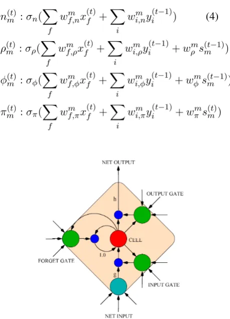
3.1 Long Short-Term Memory (LSTM) Long short-term memory (LSTM) (Hochreiter and Schmidhuber, 1997; Graves et al., 2009) is an RNN architecture specifically designed to address the vanishing gradient and exploding gradient problems. The hidden neural units are replaced by a number of memory blocks. Each memory block contains several cells, whose activations are controlled by three multiplicative gates: the input gate, forget gate and output gate. With the above change, the original rnn model is improved to be:

y_m(t) = σ(s_c,m(t) )·π_m(t) (2)

= σ(n(_mt)ρ(_mt)+φ_m(t)s(_c,mt−1))·π_m(t) (3)

Nowyis the memory block output.nis equivalent to the original hidden value yin rnn model. ρ, φ

andπare the input, forget and output gates value.

sc,mis state value of cellcin blockmandcis fixed

to be1and omitted in common work. The compu-tation of three multiplicative gates comes from in-put value, recurrent value and cell state value with different activationsσrespectively as shown in the

following and Fig. 1:

n(t)

m :σn(

X

f

wm f,nx(ft)+

X

i

wm

i,ny(it−1)) (4)

ρ(_mt):σρ(

X

f

w_f,ρm x(_ft)+X

i

w_i,ρmy(_it−1)+w_ρms(_mt−1))

φ(_mt):σφ(

X

f

wm_f,φx(_ft)+X

i

wm_i,φy_i(t−1)+wm_φs(_mt−1))

π(t)

m :σπ(

X

f

wm f,πx(ft)+

X

i

wm

i,πy(it−1)+wπms(mt))

Figure 1: LSTM memory block with a single cell. (Graves et al., 2009)

The effect of the gates is to allow the cells to store and access information over long periods of time. When the input gate is closed, the new com-ing input information will not affect the previous cell state. Forget gate is used to remove the histor-ical information stored in the cells. The rest of the network can access the stored value of a cell only when its output gate is open.

In language related problems, the structural knowledge can be extracted out by processing se-quences both forward and backward so that the complementary information from the past and the future can be integrated for inference. Thus bi-directional LSTM (B-LSTM) containing two hid-den layers were proposed(Schuster and Paliwal, 1997). Both hidden layers connect to the same in-put layer and outin-put layer, processing the same se-quence in two directions respectively (A. Graves, 2013).

LSTM layer as input, processed in reversed di-rection. These two standard LSTM layers com-pose a pair of LSTM. Then we stack LSTM layer-s pair after pair to obtain the deep LSTM model. We call this topology as deep bi-directional LSTM (DB-LSTM) network. Our experiments show that this architecture is critical to achieve good perfor-mance.

3.2 Pipeline

We process the sequence word by word. Two in-put features play an essential role in this pipeline: predicate (pred) and argument (argu), with argu-ment describing the word under processing. The output for this pair of words is their semantic role. If a sequence has np predicates, we will process

this sequencenptimes.

We also introduce two other features, predicate context (ctx-p) and region mark (mr). Since a

s-ingle predicate word can not exactly describe the predicate information, especially when the same words appear more than one times in a sentence. With the expanded context, the ambiguity can be largely eliminated. Similarly, we use region mark

mr = 1 to denote the argument position if it

lo-cates in the predicate context region, ormr = 0

if not. These four simple features are all we need for our SRL system. In Tab. 1 we give an example sequence with the labels for each word. We do not use other types of features such as part of speech (POS), syntactic parsing, etc..

time argu pred ctx-p mr label

1 A set been set . 0 B-A1

2 record set been set . 0 I-A1 3 date set been set . 0 I-A1

4 has set been set . 0 O

5 n’t set been set . 0 B-AM-NEG 6 been set been set . 1 O

7 set set been set . 1 B-V

8 . set been set . 1 O

Table 1: An example sequence with 4 input fea-tures: argument, predicate, predicate context (con-text length is 3) , region mark. “IOB” tagging scheme is used (Collobert et al., 2011).

Because the large number of parameters asso-ciated with the argument words, similar to (Col-lobert et al., 2011), the pre-trained word represen-tations are employed to address the data sparsity issue. We used a large unlabeled text corpus to train a neural language model (NLM) (Bengio et al., 2006; Bengio et al., 2003) and then

initial-ized the argument and predicate word tions with parameters from the NLM representa-tions. There are various ways of obtaining good word representations (Mikolov et al., 2013; Col-lobert and Weston, 2008; Mnih and Kavukcuoglu, 2013; Yu et al., 2014). A systematic comparison of them on the task of SRL is beyond the scope of this work.

The above four features are concatenated to be the input representation at this time step for the following LSTM layers. As described in Sec. 3.1, we use DB-LSTM topology to learn the sequence knowledge and we build up to 8 layers of DB-LSTM in our work.

As in traditional methods, we employ CRF (Lafferty et al., 2001) on top of the network for the final prediction. It takes the representations provided by the last LSTM layer as input to model the strong dependance among adjacent tags.

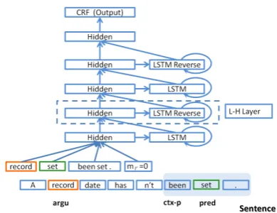
Figure 2: DB-LSTM network.Shadow part denote the predicate context within length1.

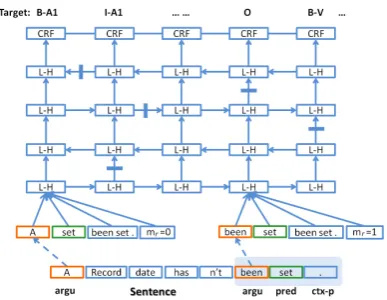
The complete model with 4 LSTM layers is il-lustrated in Fig. 2. At the bottom of the graph lo-cates the word sequence in Tab. 1. For a given time step (step2as an example), argument and predi-cate are specified with different color. We use the shadowed region to denote the predicate contex-t. The temporal expanded version of the model is shown in Fig. 3. L-H denotes the LSTM hidden layer.

Figure 3: Temporal expanded DB-LSTM network. Bars denote that the connections are blocked by the closed gates. Shadow part denotes the predi-cate context.

for CRF to perform the sequence tagging task. The traditional viterbi decoding is used for inference. The gradient of the log-likelihood of the tag se-quence with respect to the input of the CRF is cal-culated and back-propagated to all the DB-LSTM layers to get the gradient of the parameters (Col-lobert et al., 2011).

4 Experiments

We mainly evaluated and analyzed our system on the commonly used CoNLL-2005 shared task da-ta set and the conclusions are also validated on CoNLL-2012 shared task.

4.1 Data set

CoNLL-2005 data set takes section 2-21 of Wall Street Journal (WSJ) data as training set, and sec-tion 24 as development set. The test set consist-s of consist-section 23 of WSJ concatenated with 3 consist- sec-tions from Brown corpus (Carreras and M`arquez, 2005). CoNLL-2012 data set is extracted from OntoNotes v5.0 corpus. The description and sep-aration of train, development and test data set can be found in (Pradhan et al., 2013).

4.2 Word embedding

We trained word embeddings with English Wikipedia (Ewk) corpus using NLM (Bengio et al., 2006). The corpus contains 995 million to-kens. We transformed all the words into their lowercase and the vocabulary size is 4.9 million. About5%words in CoNLL 2005 data set can not be found in Ewk dictionary and are marked as

<unk>. In all experiments, we use the same word embedding with dimension32.

4.3 Network topology

In this part, we will analyze the performance of two different networks, the CNN and LSTM net-work. Although at last we find CNN can not pro-vide the results as good as that from LSTM, the analysis still help us to gain a deep insight of this problem. In CNN, we add argument context as the fifth feature and the other four features are the same as that used in LSTM. In order to have good understanding of the contribution from each mod-eling decision, we started from a simple model and add more units step by step.

4.3.1 Convolutional neural network

Using CNN to solve SRL problem has been intro-duced in (Collobert et al., 2011). Since we only focus on the analysis of features, a simplified ver-sion is used here.

Our feature set consists of five parts as de-scribed above. The representation of argument and predicate can be obtained by looking up the Emb(Ewk) dictionary. And the representation of argument context and predicate context can be ob-tained by concatenating the embedding of each word in the context. For each of the above four parts, we add a hidden layer. Then all these four hidden layers together with region mark are pro-jected onto the next hidden layer. At last we use a CRF layer for prediction (See Fig. 4). With above set up, the computational complexity isO(npL).

Figure 4: CNN Pipeline. Shadow parts denote the argument context and predicate context respec-tively

The size of hidden layers connected to argu-ment or predicate is set to beh1w = 32. The size

corresponding inputs are larger. To simplify the parameter setting and results comparison, we use the same learning ratel= 1×10−3_{for each layer} and keep this rate a constant during model train-ing. The second hidden layer dimensionh2is also

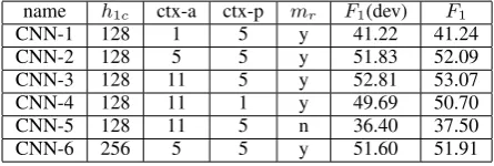
128. All hidden layer activation function istanh. In Tab. 2, it is shown that longer argument and predicate context result in better performance, since longer context brings more information. We observe the same trends in other NLP experiments, such as NER, POS tagging. The difference is that we do not need to use the context length up to11. This is because most of the useful information for NER and POS tagging is local respect the label position, while in SRL there exists long distance relationship. So in traditional methods for SRL, syntactic trees are often introduced to account for such relation. In order to see whether the improve-ment from CNN-2 to CNN-3 is due to longer con-text or larger model size, we tested a model CNN-6 with same context length but more model param-eters. As we can see from the result of CoNLL-2005 data set (Tab. 2), larger model does not im-prove the result.

name h1c ctx-a ctx-p mr F1(dev) F1

CNN-1 128 1 5 y 41.22 41.24

CNN-2 128 5 5 y 51.83 52.09

CNN-3 128 11 5 y 52.81 53.07

CNN-4 128 11 1 y 49.69 50.70

CNN-5 128 11 5 n 36.40 37.50

CNN-6 256 5 5 y 51.60 51.91

Table 2: F1 of CNN method on development set and test set of CoNLL-2005 data set.

Without using region mark (mr) feature, theF1 drops from the 53.07 of CNN-3 to the 37.50 of CNN-5. Since it is generally believed that words near the predicate are more likely to be related to the predicate.

SRL is a typical problem with long distance de-pendency, while the convolution operation can on-ly learn the knowledge from the limited neighbor-hood. This is why we have to introduce long con-text. However, the language information can not be expressed just by linearly expanding the con-text as what we did in CNN pipeline. In order to better summarize the sequence structure, we turn to LSTM network.

4.3.2 LSTM network

Here the feature set consists of four parts. Ar-gument and predicate are necessary parts in this

problem. In recurrent model, argument context (ctx-a) is no longer needed and we only expand the predicate context. We also need the region mark defined in the same way as in CNN. The archi-tecture has been shown in Fig. 2 and described in Sec. 3.2.

Since it is difficult to propagate the error from the top to the bottom layers, we use two learning rates. At the bottom,i.e.from embeddings to the first LSTM layer, we uselb = 1×10−2for

mod-el depthd <= 4andlb = 2×10−2 ford > 4.

For the other LSTM layers and CRF layer, we set learning rate l = lb ×10−3. We kept all

learn-ing rates constant durlearn-ing trainlearn-ing. The model size can be enlarged by increasing the number of LST-M layers (d) or the dimension of hidden layers (h). L2 weight decay in SGD is used for model regu-larization and we set its strengthr2= 8×10−4:

w←w−l·(g+r2·w) (5)

wherewdenotes the parameter,g the gradient of the log likelihood of the label with respect to the parameter.

We started on CoNLL-2005 dataset from a small model with only one LSTM layer andh = 32. All word embeddings were randomly initial-ized. Predicate context length was 1. Region mark is not used. With this model, we obtained

F1 = 49.44(Tab. 3), better than that of CNN with-out using argument context (41.24) or region mark (37.50). This result suggests that, the recurrent structure can extract sequential information more effectively than CNN.

By adding predicate context with length5, F1 is improved from49.44to56.85(Tab. 3). This is because we only recurrently process the argument word, so we still need predicate context for more detail. Further more, F1 rises to 58.71 with re-gion mark feature. The reason is the same as we explained in CNN pipeline.

Next we change the random initialization of word representation to the pre-trained word rep-resentation from Emb(Ewk). This reprep-resentation is fixed in the training process. F1 rises to65.11 (See Tab. 3).

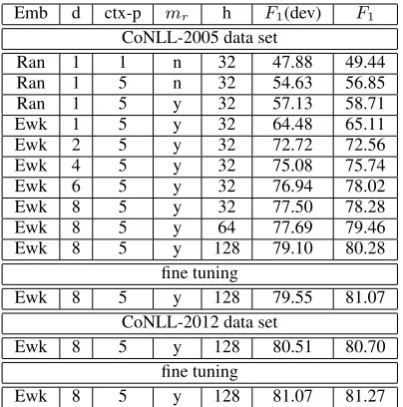
Emb d ctx-p mr h F1(dev) F1 CoNLL-2005 data set

Ran 1 1 n 32 47.88 49.44

Ran 1 5 n 32 54.63 56.85

Ran 1 5 y 32 57.13 58.71

Ewk 1 5 y 32 64.48 65.11

Ewk 2 5 y 32 72.72 72.56

Ewk 4 5 y 32 75.08 75.74

Ewk 6 5 y 32 76.94 78.02

Ewk 8 5 y 32 77.50 78.28

Ewk 8 5 y 64 77.69 79.46

Ewk 8 5 y 128 79.10 80.28

fine tuning

Ewk 8 5 y 128 79.55 81.07

CoNLL-2012 data set

Ewk 8 5 y 128 80.51 80.70

fine tuning

Ewk 8 5 y 128 81.07 81.27

Table 3: F1 with LSTM method on development set and test set of CoNLL-2005 data set and CoNLL-2012 data set. Emb: the type of embed-ding. d: the number of LSTM layers. ctx-p: pred-icate context length. mr: region mark feature. h:

hidden layer size.

We find that the critical improvement comes from increasing the depth of LSTM network. Af-ter adding a reversed LSTM layer,F1is improved from 65.11 to 72.56. And the F1 of the system with d = 4,6,8 are 75.74,78.02 and 78.28 re-spectively. With6-layer network, we have outper-formed the CoNLL-2005 shared task winner sys-tem withF1 = 77.92(Koomen et al., 2005). Our experiment results also show that the further per-formance gain by increasing the depth from 6 to 8 is relative small.

Another way to increase the model size is to in-crease the hidden layer dimensionh. We gradually increase the dimension from32to64,128, and the corresponding results are listed in Tab. 3. The best

F1 we obtained is 80.28 with h = 128. We al-so show the result F1 = 80.70 on CoNLL-2012 dataset in Tab. 3 with exactly the same setup.

In the above experiments, learning rate and weight decay rate are fixed for the sake of sim-plicity in comparing different models. To fur-ther improve the model, we perform a fine tuning step to adjust the parameters based on previous-ly trained model. This includes the relaxation of weight decay and decrease of learning rate. We setr2 = 4×10−4andlb = 1×10−2, and obtain

F1= 81.07as the final result of CoNLL-2005 da-ta set andF1 = 81.27of CoNLL-2012 data set.

F1 F1

CoNLL-2005 dev test WSJ Brown

Koomen 77.35 77.92 79.44 67.75

Koomen (single parser) 74.76 - -

-Pradhan 78.34 77.30 78.63 68.44

Collobert (w/ parser) 75.42 76.06 - -Collobert (w/o parser) 72.29 74.15 -

-Surdeanu - - 80.6 70.1

Toutanova 78.6 - 80.3 68.8

T¨ackstr¨om 78.6 - 79.9 71.3

Ours 79.55 81.07 82.84 69.41

F1 F1

CoNLL-2012 dev test -

-Pradhan - 75.53

T¨ackstr¨om 79.1 79.4

Ours 81.07 81.27

Table 4: Comparison with previous methods.

In Tab. 4, we compare the performance of oth-er works. On CoNLL-2005 shared task, moth-erg- merg-ing syntactic tree at feature level instead of model level exhibits the similar performance withF1 =

77.30(Pradhan et al., 2005). After further investi-gation on model combination, Surdeanu et al. ob-tained a better system (Surdeanu et al., 2007). We also list the results from (Toutanova et al., 2008) and (T¨ackstr¨om et al., 2015) of the joint model with additional considerations of standard linguis-tic assumptions. For convolution based methods (Collobert et al., 2011), the best F1 is 76.06, in which syntactic parser plays an essential role. The result without using parser drops down to 74.15. On Brown set, we observe the better performance from the work of (Surdeanu et al., 2007) and (T¨ackstr¨om et al., 2015). We hypothesize that DB-LSTM is a data-driven method that can not per-forms well on out-domain dataset.

On CoNLL-2012 data set, the traditional method gives F1 = 75.53(Pradhan et al., 2013) and a dynamic programming algorithm for effi-cient constrained inference in SRL gives F1 =

79.4(T¨ackstr¨om et al., 2015) , both of them also rely on syntax trees.

Since the input feature size is much smaller then the traditional sparse feature templates, the infer-ence stage is very efficient that the model can pro-cess6.7k tokens per second on average.

4.4 Analysis

Results (Koomenet.al.) Results (Ours)

Data set P R F1 P R F1

dev 80.05 74.83 77.35 79.69 79.41 79.55 dev (s) 75.40 74.13 74.76 79.69 79.41 79.55 test WSJ 82.28 76.78 79.44 82.92 82.75 82.84 test Brown 73.38 62.93 67.75 70.70 68.17 69.41 test 81.18 74.92 77.92 81.33 80.80 81.07 A0 88.22 87.88 88.05 90.08 89.73 89.91 A1 82.25 77.69 79.91 82.00 82.87 82.43 A2 78.27 60.36 68.16 70.50 72.63 71.55 A3 82.73 52.60 64.31 63.98 55.68 59.54 AM-ADV 63.82 56.13 59.73 66.03 53.00 58.80 AM-DIS 75.44 80.62 77.95 73.76 78.07 75.85 AM-LOC 66.67 55.10 60.33 65.17 58.48 61.65 AM-MNR 66.79 53.20 59.22 56.36 54.63 55.48 AM-MOD 96.11 98.73 97.40 94.62 98.60 96.57 AM-NEG 97.40 97.83 97.61 95.70 95.36 95.53 AM-TMP 78.16 76.72 77.44 78.61 82.74 80.62 R-A0 89.72 85.71 87.67 94.72 93.57 94.14 R-A1 70.00 76.28 73.01 80.00 90.40 84.88 V 98.92 97.10 98.00 98.63 98.63 98.63

Table 5:F1on each sub sets and classes (CoNLL-2005). (We remove the classes with low statistics.)

final system is the combination of the results of

5 parsing trees from two different parsers. They also reported the scores of each single system on development set and we list the best one of them (dev(s)).

We observe the improvement ofF1on develop-ment set and test set are2.20and3.15 respective-ly. For single system, the improvement is4.79on development set. We also notice that our model show improvement on both WSJ and Brown test set. The advantage of our model is even more sig-nificant when comparing with the previous effort of end-to-end training of SRL model (Collobert et al., 2011). Without using linguistic features from parse tree, the F1 of Collobert’s model is74.15, which is6.92lower than our model.

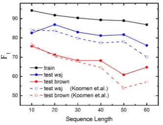
Figure 5:F1vs. sentence length (CoNLL-2005).

In order to analyze the performance of our mod-el on the sentences with different lengths, we split the data into 6 bins according to the sentence length, with bin width being10words and the last

bin includes sequences withL >50because of in-sufficient data for longer sentences. Fig. 5 shows

F1 scores at different sequence lengths on WSJ test data and Brown test data for our model and Koomen’s model (baseline) (Koomen et al., 2005). In all curves, performance degrades with increased sentence length. However, the performance gain of our model over the baseline model is larger for longer sentences.

Figure 7: Averaged Forget gates value vs. Syn-tactic distance (CoNLL-2005). The last point in-cludes instances with syntactic distanceds≥6.

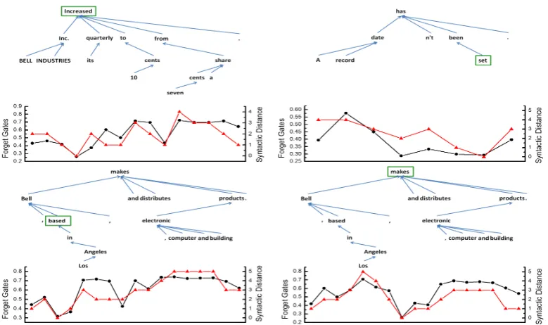
Since we do not use any syntactic information as input feature, we are curious about whether this information can be extracted out from the system parameters. In LSTM, forget gates are used to control the use of historical information. We com-pute the average valuevfg of forget gates of the

7th _{LSTM layer at word position for a given}

sen-tence. We also introduce a variable named syntac-tic distance ds to represent the number of edges

between argument word and predicate word in the dependency parsing tree. Four example sentences are shown in Fig. 6. For each figure, the bottom axis denotes an example sentence. At the top of each graph is the corresponding dependency tree built from gold dependency parsing tag. At the bottom, vfg and ds are shown in black and red

line. Noticed that the higher forget gates values means “Remember” and smaller values “Forget”. Smallerdsmeans that it is easy to make prediction

that long history is unnecessary. On the contrary, large ds results in a difficult prediction that long

historical information is needed. We also com-puted the averagevfg over instances and found it

monotonously increases withds(Fig. 7). The

co-incidence of vfg and ds suggests that the model

implicitly captures some syntactic structure.

5 Conclusion and Future work

Figure 6: Forget gates valuevs. Syntactic distance on four example sentences. Top: dependency parsing tree from gold tag. Green square word: predicate word. Bottom black solid lines: forget gates value at each time step. Bottom red empty square lines: gold syntactic distance between the current argument and predicate.

able to bypass the traditional steps for extracting the intermediate NLP features such as POS and syntactic parsing and avoid human engineering the feature templates. The model is trained to predict the SRL tag directly from the original word se-quence with four simple features without any ex-plicit linguistic knowledge. Our model achieves

F1 score of 81.07 on CoNLL-2005 shared task and81.27on CoNLL-2012 shared task, both out-performing the previous systems based on parsing results and feature engineering, which heavily re-ly on the linguistic knowledge from expert. Fur-thermore, the simplified feature templates results in high inference efficiency with6.7ktokens per second.

In our experiments, increasing the model depth is the major contribution to the final improvement. With deep model, we achieve strong ability of learning semantic rules without worrying about over-fitting even on such limited training set. It al-so outperforms the convolution method with large context length. Moreover, with more sophisti-catedly designed network and training technique based on LSTM, such as the attempt to integrate the parse tree concept into LSTM framework (Tai et al., 2015), we believe the better performance can be achieved.

We show in our analysis that for long sequences

our model has even larger advantage over the tra-ditional models. On one hand, LSTM network is capable of capturing the long distance dependen-cy especially in its deep form. On the other hand, the traditional feature templates are only good at describing the properties in neighborhood and a small mistake in syntactic tree will results in large deviation in SRL tagging. Moreover, from the analysis of the internal states of the deep network, we see that the model implicitly learn to capture some syntactic structure similar to the dependen-cy parsing tree.

References

G. Hinton A. Graves, A. Mohamed. 2013. Speech recognition with deep recurrent neural network-s. InIEEE International Conference on Acoustics, Speech, and Signal Processing, ICASSP 2013. Emanuele Bastianelli, Giuseppe Castellucci, Danilo

Croce, and Roberto Basili. 2013. Textual inference and meaning representation in human robot interac-tion. InProceedings of the Joint Symposium on Se-mantic Processing. Textual Inference and Structures in Corpora, pages 65–69.

Yoshua Bengio, Patrice Simard, and Paolo Frasconi. 1994. Learning long-term dependencies with gradi-ent descgradi-ent is difficult. IEEE Transactions on Neu-ral Networks, 5(2):157–166.

Yoshua Bengio, R´ejean Ducharme, Pascal Vincent, and Christian Janvin. 2003. A neural probabilistic lan-guage model. Journal of Machine Learning Re-search, 3:1137–1155, March.

Yoshua Bengio, Holger Schwenk, Jean-Sbastien Sen-cal, Frderic Morin, and Jean-Luc Gauvain. 2006. Neural probabilistic language models. In Innova-tions in Machine Learning, volume 194 ofStudies in Fuzziness and Soft Computing, pages 137–186. Springer Berlin Heidelberg.

Xavier Carreras and Llu´ıs M`arquez. 2005. Intro-duction to the CoNLL-2005 shared task: Semantic role labeling. In Proceedings of the Ninth Confer-ence on Computational Natural Language Learning (CoNLL-2005), pages 152–164, Ann Arbor, Michi-gan, June. Association for Computational Linguis-tics.

Eugene Charniak and Mark Johnson. 2005. Coarse-to-fine n-best parsing and maxent discriminative r-eranking. InProceedings of the 43rd Annual Meet-ing on Association for Computational LMeet-inguistics, ACL ’05, pages 173–180, Stroudsburg, PA, USA. Association for Computational Linguistics.

Eugene Charniak. 2000. A

maximum-entropy-inspired parser. In Proceedings of the 1st North American Chapter of the Association for Computa-tional Linguistics Conference, NAACL 2000, pages 132–139, Stroudsburg, PA, USA. Association for Computational Linguistics.

Michael Collins. 2003. Head-driven statistical mod-els for natural language parsing. Comput. Linguist., 29(4):589–637, December.

Ronan Collobert and Jason Weston. 2008. A unified architecture for natural language processing: Deep neural networks with multitask learning. In Pro-ceedings of the 25th International Conference on Machine Learning, ICML ’08, pages 160–167, New York, NY, USA. ACM.

Ronan Collobert, Jason Weston, L´eon Bottou, Michael Karlen, Koray Kavukcuoglu, and Pavel Kuksa.

2011. Natural language processing (almost) from scratch. Journal of Marchine Learning Research, 12:2493–2537, November.

Shen Dan and Mirella Lapata. 2007. Using seman-tic roles to improve question answering. In Pro-ceedings of the 2007 Joint Conference on Empirical Methods in Natural Language Processing and Com-putational Natural Language Learning (EMNLP-CoNLL).

Alex Graves, Marcus Liwicki, Santiago Fernan-dez, Roman Bertolami, Horst Bunke, and J¨urgen Schmidhuber. 2009. A novel connectionist system for unconstrained handwriting recognition. IEEE Transactions on Pattern Analysis and Machine In-telligence, 31(5):855–868.

Alex Graves, Greg Wayne, and Ivo Danihelka. 2014. Neural turing machines. arXiv:1410.5401.

S. Hochreiter and J. J¨urgen Schmidhuber. 1997. Long short-term memory. Neural Computation, 9(8):1735–1780.

Yoon Kim. 2014. Convolutional neural networks for sentence classification. InProceedings of the 2014 Conference on Empirical Methods in Natural Lan-guage Processing, pages 1746–1751.

Peter Koomen, Vasin Punyakanok, Dan Roth, and Wen-tau Yih. 2005. Generalized inference with multiple semantic role labeling systems. In Pro-ceedings of the 9th Conference on Computation-al NaturComputation-al Language Learning, CONLL ’05, pages 181–184, Stroudsburg, PA, USA. Association for Computational Linguistics.

John D. Lafferty, Andrew McCallum, and Fernando C. N. Pereira. 2001. Conditional random fields: Probabilistic models for segmenting and labeling se-quence data. InProceedings of the 8th International Conference on Machine Learning, ICML ’01, pages 282–289, San Francisco, CA, USA. Morgan Kauf-mann Publishers Inc.

Yann Lecun, Lon Bottou, Yoshua Bengio, and Patrick Haffner. 1998. Gradient-based learning applied to document recognition. InProceedings of the IEEE, pages 2278–2324.

Tomas Mikolov, Ilya Sutskever, Kai Chen, Greg Cor-rado, and Jeffrey Dean. 2013. Distributed represen-tations of phrases and their compositionality. In Ad-vances on Neural Information Processing Systems. Andriy Mnih and Koray Kavukcuoglu. 2013. Learning

word embeddings efficiently with noise-contrastive estimation. InAdvances in Neural Information Pro-cessing Systems, pages 2265–2273.

Martha Palmer, Daniel Gildea, and Nianwen Xue. 2010. Semantic Role Labeling. Synthesis Lec-tures on Human Language Technology Series. Mor-gan and Claypool.

Jacob Persson, Richard Johansson, and Pierre Nugues. 2009. Text categorization using predicatecargumen-t spredicatecargumen-trucpredicatecargumen-tures. InProceedings of NODALIDA, pages 142–149.

Sameer Pradhan, Kadri Hacioglu, Wayne Ward, James H. Martin, and Daniel Jurafsky. 2005. Se-mantic role chunking combining complementary syntactic views. InProceedings of the 9th Confer-ence on Computational Natural Language Learning, CONLL ’05, pages 217–220, Stroudsburg, PA, US-A. Association for Computational Linguistics.

Sameer Pradhan, Alessandro Moschitti, Nianwen Xue, Hwee Tou Ng, Anders Bj¨orkelund, Olga Uryupina, Yuchen Zhang, and Zhi Zhong. 2013. Towards ro-bust linguistic analysis using ontonotes. In Proceed-ings of the Seventeenth Conference on Computa-tional Natural Language Learning, pages 143–152, Sofia, Bulgaria, August. Association for Computa-tional Linguistics.

V. Punyakanok, D. Roth, and W. Yih. 2008a. The importance of syntactic parsing and inference in se-mantic role labeling. Computational Linguistics, 34(2).

Vasin Punyakanok, Dan Roth, and Wen tau Yih. 2008b. The importance of syntactic parsing and inference in semantic role labeling. Computational linguistics, 6(9).

M. Schuster and K. K. Paliwal. 1997. Bidirection-al recurrent neurBidirection-al networks. IEEE Transactions on Signal Processing, 45:2673–2681.

Mihai Surdeanu, Sanda Harabagiu, John Williams, and Paul Aarseth. 2003. Using predicate-argument structures for information extraction. In Proceed-ings of the 41st Annual Meeting on Association for Computational Linguistics - Volume 1, ACL ’03, pages 8–15, Stroudsburg, PA, USA. Association for Computational Linguistics.

Mihai Surdeanu, Llu´ıs M`arquez, Xavier Carreras, and Pere R. Comas. 2007. Combination strategies for semantic role labeling. Journal of Artificial Intelli-gence Research, 29:105–151.

Ilya Sutskever, Oriol Vinyals, and Quoc V Le. 2014. Sequence to sequence learning with neural network-s. In Advances on Neural Information Processing Systems.

Oscar T¨ackstr¨om, Kuzman Ganchev, and Dipanjan Das. 2015. Efficient inference and structured learn-ing for semantic role labellearn-ing. Transactions of the Association for Computational Linguistics, 3:29–41.

Kai Sheng Tai, Richard Socher, and Christopher D. Manning. 2015. Improved semantic representation-s from tree-representation-structured long representation-short-term memory net-works. InProceedings of the 53st Annual Meeting on Association for Computational Linguistics, ACL ’15, Stroudsburg, PA, USA. Association for Compu-tational Linguistics.

Kristina Toutanova, Aria Haghighi, and Christopher D. Manning. 2008. A global joint model for semantic role labeling. Computational Linguistics, 34:161– 191.

Oriol Vinyals, Lukasz Kaiser, Terry Koo, Slav Petrov, Ilya Sutskever, and Geoffrey Hinton. 2014. Gram-mar as a foreign language. arXiv:1412.7449. Jason Weston, Sumit Chopra, and Antoine Bordes.

2014. Memory networks.arXiv:1410.3916. Jason Weston, Antoine Bordes, Sumit Chopra, and

Tomas Mikolov. 2015. Towards ai-complete ques-tion answering: A set of prerequisite toy tasks. arX-iv:1502.05698.

Mo Yu, Matthew Gormley, and Mark Dredze. 2014. Factor-based compositional embedding models. In

Advances in Neural Information Processing Systems Workshop on Learning Semantics.