Estimation of Open Channel Flow Parameters by Using Genetic Algorithm

(1)

ISSN Print: 2325-7105

DOI: 10.4236/ojop.2018.73003 Sep. 30, 2018 51 Open Journal of Optimization

Estimation of Open Channel Flow Parameters

by Using Genetic Algorithm

Ebissa Gadissa, Asirat Teshome

Department of Hydraulic and Water Resources Engineering, Debre Tabor University, Debre Tabor, Ethiopia

Abstract

The present study involves estimation of open channel flow parameters hav-ing different bed materials invokhav-ing data of Gradual Varied Flow (GVF). Use of GVF data facilitates estimation of flow parameters. The necessary data base was generated by conducting laboratory. In the present study, the efficacy of the Genetic Algorithm (GA) optimization technique is assessed in estimation of open channel flow parameters from the collected experimental data. Computer codes are developed to obtain optimal flow parameters Optimiza-tion Technique. Applicability, adequacy and robustness of the developed code are tested using sets of theoretical data generated by experimental work. A simulation model was developed to compute GVF depths at preselected dis-crete sections for given downstream head and discharge rate. This model is linked to an optimizer to estimate optimal value of decision variables. The proposed model is employed to a set of laboratory data for three bed mate-rials. Application of proposed model reveals that optimal value of fitting pa-rameter ranges from 1.42 to 1.48 as the material gets finer and optimal deci-sion variable ranges from 0.015 to 0.024. The optimal estimates of Manning’s n of three different bed conditions of experimental channel appear to be higher than the corresponding reported/Strickler’s estimates.

Keywords

Parameter Estimation, Genetic Algorithm, Optimal Values, GVF Profiles

1. Introduction

Parameter identification techniques have been widely used in the field of hy-drology, meteorology, and oceanography. [1] used the adjoint equation method to identify a profile of Manning’s n in an idealized trapezoidal open channel. In Addition to this, [1] used Lagrangian multipliers and a least square error

crite-How to cite this paper: Gadissa, E. and Teshome, A. (2018) Estimation of Open Channel Flow Parameters by Using Genetic Algorithm. Open Journal of Optimization, 7, 51-64.

https://doi.org/10.4236/ojop.2018.73003

Received: September 1, 2018 Accepted: September 27, 2018 Published: September 30, 2018

(2)

DOI: 10.4236/ojop.2018.73003 52 Open Journal of Optimization

rion to estimate roughness coefficients. Research involving the GMS equation traditionally focuses on the determination of the roughness coefficient, (n), un-der different flow regimes [2]. Optimization techniques were successfully used by [3], to identify parameters for regular prismatic channels having simple cross-sections.

The issue of parameter identification based on the optimal control theories in oceanography can be traced from the early work of [4], carried out early an ad-joint parameter identification for bottom drag coefficient in a tidal channel. An effective methodology has been proposed to evaluate optimal design of cross sectional area of a channel having composite roughness using Manning’s roughness equation. [5] [6] estimated the bottom friction and water depth in a two-dimensional tidal flow. More recently, [7] used the quasi-Newton method to identify Manning’s roughness coefficients in shallow water flows. Nevertheless, the above studies considered only the case of in-bank flow. Therefore, there is a need to extend the method to out-bank flow, where flood plain roughness will obviously have to be considered.

Genetic algorithms are computationally simple yet powerful search algorithms that seek to produce mathematically the mechanics of natural selection and nat-ural genetics, according to the biological processes of survival and adaptation.

[8] [9] identified a constant Manning’s n in an open channel flow with a mova-ble bed. [10] identified the friction parameter in 1D open channel considering the selection of performance function and effect of uncertainty in observed data. And also [10] used a nonlinear least square technique with three types of objec-tive function and identified open channel friction parameters by a modified Gauss-Newton method.

Genetic programming (GP—an extension of genetic algorithms to the domain of computer programs [11]), a technique generated from the seminal work of numerous researchers in the 1970s and 1980s, generates possible solutions that fit Manning and Albert Strickler. A superior algorithm was proposed for the tree type network which involves the segmentation of channel network into small parts followed by their individual solution using forth order Runge-Kutta me-thod and linking the solution of smaller units to yield the solution of entire channel network by applying shooting method [12].

One of the very few studies which dealt with the identification of compound channel flow parameters is the one by [13]. In this study, roughness coefficients in the main channel and flood plains were identified as two different parameters using an automatic optimization method. The model was applied to Duong Riv-er in Vietnam, whRiv-ere roughness coefficients of the main channel and the flood plain were presented as different constant values as well as polynomial functions of stage. [14] solved the inverse problem of identifying the roughness coefficient in a channel network using the sequential quadratic programming algorithm.

(3)

af-DOI: 10.4236/ojop.2018.73003 53 Open Journal of Optimization

fect the surface roughness, runoff and erodibility of the channel [15] [16], esti-mated flood discharges using the Levenberg–Marquardt minimization algo-rithm.

Therefore, the objectives his study are to: 1) identify open channel flow para-meters by using Genetic Algorithm optimization Technique, 2) generate and monitor gradually varied flow profiles corresponding to different bed materials, discharge and ponded depths, 3) Invoking the observed data of the GVF profiles and the linked simulation optimization approach to estimates Manning’s n cor-responding to different channel bed materials in the experimental channel, and 4) minimize errors by using optimization methods.

2. Methods and Materials

2.1. Methods

This study was carried out to identify open channel flow parameters by using Genetic Algorithm optimization technique. Manning’s roughness coefficient and other parameters are estimated for different bed materials used (d50 = 8 mm and

d50 = 25 mm grain size and Lined concrete bed materials). Also, GVF flow

pro-file is identified. Crank-Nicolson method is used to solve the governing differen-tial equation. Parameter optimization technique is used to find the optimal value of coefficient roughness for three different bed materials. Estimation of rough-ness coefficient is based on Manning’s equation for estimation of manning roughness coefficient and corresponding manning roughness parameters. This estimation invokes the data of observed GVF profiles and such accounts for dif-ferent bed materials with the flow depth. Experimental works is done to several sets of data monitored in Hydraulics Laboratory of Civil Engineering Depart-ment.

2.2. Materials

Flume

A rectangular tilting flume of length 30 m, width 0.205 m and height 0.50 m was used. The bed of the flume was made up of lined concrete and the other two sides were made up of glass and GI sheet. Discharge was released through an in-let pipe of 0.010 m diameter into the flume. The entrance of the channel was provided with flow suppressors in order to make the flow stable. In order to maintain desired depth of water at the downstream of the channel, a tail gate was fitted at the end of the channel. Water discharging from the tail gate, passed to the sump which was circulated again through a 15 hp centrifugal pump for fur-ther experimentation.

Experimental Procedures

The experiments were conducting by adopting the following steps as men-tioned below:

Slope Measurement

(4)

The slope was measured by using two steel containers connected with a long rubber tube. Both the containers were placed on the channel bed separated by the rubber tube along the length of the channel. One of the containers placed at higher elevation was filled with water and simultaneously care was taken to re-move air bubble from the connecting tube. They are left undisturbed for suffi-cient amount of time around 24 hours. Then the water levels were measured. Then, slope of the channel was computed.

Sieve Analysis

Sieve analysis was performed to determine the particle size of the material used to create artificial bed roughness. Results of sieve analysis were plotted to investigate the particle size of the bed material used in the present study. Expe-riments were conducted on two different bed materials. First on one rough bed condition having gravel as a bed particle size d50 = 25 mm, d50 = 8 mm and then

on the smooth condition having lined concrete as bed material. The sieve analy-sis of aggregate is done by a set of standard sieves. The procedure of determina-tion is presented below. Total mass of sample is 1kg (Look Figure 1 and Figure 2).

Calibration of orifice meter

[image:4.595.241.508.447.557.2]

Orifice meter was provided in the inlet pipe for the measurement of discharge. Orifice plate was made up of GI sheet having diameter of 0.06 m and the diame-ter of inlet pipe was 0.10 m. Ultrasonic flow mediame-ter was used for the calibration of coefficient of discharge of orifice meter. Different discharges were noted corres-ponding to varying head. This result was plotted and the best fitted line was used.

Figure 1. Gradation curve for d50 = 25 mm.

[image:4.595.239.513.592.705.2]

(5)

Measurement of water surface profiles

1) Water was released into the rectangular flume by opening the valve of inlet pipe.

2) The desired depth of flow was maintained at the downstream end by oper-ating sluice gate provided at the end of the channel. The depth of water was measured using pointer gauge.

3) After a while when the flow become steady in the channel and the desired depth was maintained at the downstream end, the water surface profile was be-ing measured.

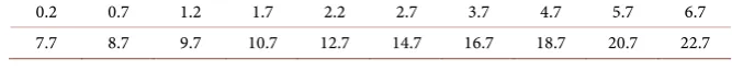
4) Starting from the maintained depth at the downstream end (0.00 m), the water surface profile is measured towards upstream at ten (21) discrete locations that are 0.00 m, 0.20 m, 0.70 m, 1.20 m, 1.70 m, 2.20 m, 2.70 m, 3.70 m, 4.70 m, 5.70 m, 6.70 m, 7.70 m, 8.70 m, 9.70 m, 10.70 m, 12.70 m, 14.70 m, 16.70 m, 18.70 m, 20.70 m and 22.70 m.

5) The above mentioned steps were repeated for three different downstream depths, Discharges rates and bed roughness are mentioned in Tables.

Collection of data

The data obtained for experimental measured water surface profiles corres-ponding to different bed materials is presented in Tables ford50 = 25 mm, d50 = 8

mm and lined concrete respectively.

Genetic Algorithms& Model Description

Optimization techniques were successfully used by [17], to identify parame-ters for regular prismatic channels having simple cross-sections. These research-ers used the same optimization algorithm (the so-called “Influence Coefficient” Algorithm) which, mathematically, is closely related to both quasi linearization and the gradient method.

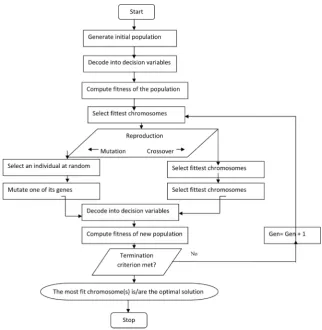
Genetic Algorithm combines survival of the fittest among string structures (used to represent the specific entity to be optimized) with a structured, yet randomized information exchange to form a search algorithm. In every genera-tion, a new set of artificial entities (or strings) is created using bits and pieces of the fittest of the old; an occasional new part is tried for good measure. While randomized, Gas are no simple random walk. They efficiently exploit historical information to speculate on new search points, with expected new performance. GAs, in essence, are heuristic (nonexact), probabilistic (stochastic), combina-torial (discrete), search based optimization technique and the continuing price or performance improvements of computational systems have made them at-tractive for various types of optimization problems.

(6)

[image:6.595.212.535.376.707.2]

solving a particular problem has five major components, which are succinctly described in the succeeding sections. A general flowchart of GA is shown in

Figure 3.

Simulation Model

The optimization problem posed in the preceding section is solved by em-ploying the linked optimization problem. This approach would require devel-opment of a model for simulation of GVF depths at preselected discrete sections for given downstream head and discharge rate. Subsequently this simulation model is linked to an optimizer for addressing the optimization problem. Effec-tively the simulation model would provide the vector of computed depths

(

_i, ,_k _i

)

y x Q H appearing in the objective function. The details of the simulation model in the following sections.

Discretization of reach

In the simulation model the entire channel reach is discretized into M small space steps such that depth of water level at Mth_{step is greater than 1.01 ×}

nor-mal depth.

Governing differential equation

Some advanced numerical techniques like standard forth order Runge-Kutta method, Kutta-Merson method etc. are also used to solve the governing diffe-rential equation of the flow.

(7)

Governing differential equation used for simulation of GVF is given as:

2 3 d d ₁ o f S S y

x Q T

gA

− =

−

(1)

In this equation d

d

y

x is change in depth y with distance x; Sf is energy slope and T is top width. Sf can be calculated by using Manning’s formula as:

2 2

2 4 3c

f n Q

S A R

= ₍₂₎

where nc is composite roughness coefficient given by Equation (8).

Simulation strategy

Crank-Nicolson method is used to solve the governing differential equation mentioned in above section. In this method, depth of water level at next space step is calculated as:

1

i i

y₊ =y − ∆β x₍₃₎

where, yi+1 and yi is depth of water level at i + 1th and ith section respectively,

x

∆ _{is the distance between them and} β _{is the average slope which is given as} follow: 1 d d d d 2 i i

y _y y _y

x x

β

+

= (4)

where, d_dy y_x i

 

 

  and 1

d dy y_x i+

 

 

  are the change in the depth of flow with

channel distance x at ith_and_i₊₁th_{section. Equation (3) can be further elaborated}

using previously mentioned equation as:

2 2 2 2

2 10 3 2 10 3

1

2 2

2 3 2 3

1 1 1 1 2 ci ci o o i i i i i i

n Q n Q

S S x

T y T y

Q Q

gT y gT y

y y + + +         − − ∆    ₊    − −    

= − ₍₅₎

where, nci and nci+1 are the composite roughness of ith and i + 1th section. An

iterative procedure is adopted for the computation of yi+1. In this procedure, 1

1

l i y+

+ is calculated where l is the number of iteration as:

1 1

l

i i

y+ y β x

+ = − ∆ (6)

And the iteration ends when it met the converging criterion, which is given as:

1

1 1

l l

i i

y+ y

+ − + < ∈ (7)

where, ∈ is a constant term. Thus, using the above mentioned approach yi+1

is computed for each discrete step up to Mth_{step and this leads to the simulation}

(8)

2.3. Model Application

Data Base

As discussed, the laboratory channel is rectangular in section with roughening bed material lying on the bed width and the two sides made up of glass and GI sheet. Thus there are three segments of wetted perimeter i.e. bed and two sides one of glass and other of GI sheet. The experiments were performed for three types of bed conditions and several sets of discharge rates downstream head as enumerated in Table 1.

The depths were measured at 20 locations upstream of the control section. The co-ordinates of the locations (measured upstream of the control section) are shown in Table 2.

Simulator

Multi roughness channels are not uncommon in field application of open channel flow hydraulics. [18], used singular value decomposition to calibrate the Manning’s roughness in one-dimensional (1D) Saint Venant equations. Due to different roughness of wetted perimeter the overall roughness of the channel is given by composite roughness. Composite roughness comprises of individual roughness effect of channel cross section. Seventeen different equations based on several assumptions along with six different techniques to sub divide the channel cross section were given by numerous investigators [19]. The credibility of these equations would be assessed by employing experimental data.

[image:8.595.244.499.467.566.2]

As mentioned below (For composite channel roughness look Figure 4), the experimental channel consists of three types of wetted perimeter; accordingly following equation is used in the simulator for computing the composite rough-ness nc:

[image:8.595.209.540.621.664.2]

Figure 4. Composite channel roughness.

Table 1. Data used for experimental measurement of water surface profiles.

Discharge rates (m3_/s) _{9.50 × 10}−3 _{1.25 × 10}−3 _{1.45 × 10}−3 Downstream depths (m) 0.25 m 0.30 m 0.35 m Bed materials (d50 in mm) d50 = 25 mm d50 = 8 mm Lined concrete

Table 2. Co-ordinates of the locations of observed GVF profiles (measured in meter).

[image:8.595.205.539.699.737.2]

(9)

(

)

(

)

1 2 3

1

1 2

c

n B n y n y

n

B y

∝

∝ ∝ ∝

∝

∗ + ∗ + ∗

=

+ (8)

where, nc is the composite Manning’s n, n1, n2, and n3 are value of

Man-ning’s n for bed and sides respectively. B is bed width and y is the depth of flow. Since composite roughness depends on the depth of the flow, which is not con-stant in the present scenario. Therefore, nc is computed at each section of the

water surface flow profile. The value of ∈ is take n as 0.001 in Equation (11). Optimization

The following problem was solved three times corresponding to different bed conditions i.e.d50 = 25 mm, d50 = 8 mm and lined concrete as bed materials.

Decision Variables:

(

n i_i, =1,2,3

)

_{; and} ∝_. Objective Function:

(

)



2

3 3

Min M i i, ,k l ikl

l k i

Z = w y x Q H −y 

 

 

∑∑∑

(9)

where, y x Q H

(

_i, ,_k _l

)

and yikl are simulated and experimentally measured

depth at ith_{discrete section,}_kth_{discharge rate and}_lth_{downstream head}

respec-tively; M is a subset of the locations where the observed depth is larger than 1.01 x normal depth; wi is the weight assigned to the mismatch at ith location. In the

present study the weights are assigned to index the length discretized by the dis-crete sections. Thus (wi) is defined as follows:

(

1 1

)

2

i i

i

x x

w ₌ + − − ₍₁₀₎

Constraint:

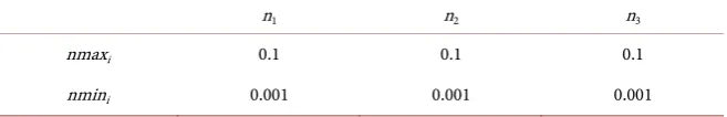
1) Following six constraints were assigned to impose upper and lower limits of the segment roughness coefficients (nmaxi and nmini, i = 1, 2, 3).

, 1,2,3

i i

nmax nmin i≥ = ₍₁₁₎ The adopted values of the limits are given in Table 3.

2) Following three constraints were assigned to ensure realistic relative roughness of the three roughness coefficients.

1 2 3

n n≥ ≥n ₍₁₂₎

3) Following constraints was assigned to impose upper and limits of fitting parameters (∝).

[image:9.595.211.540.672.725.2]

2≥ ∝ ≥1₍₁₃₎

Table 3. Upper and lower limits of roughness coefficients.

n1 n2 n3

nmaxi 0.1 0.1 0.1

(10)

Since the reported value of ∝_{1.5, a range of 1 to 2 was prescribed.}

Linked simulation optimization approach is used to estimate the optimal val-ues of the parameters for three bed conditions i.e.d50 = 25 mm, d50 = 8 mm and

lined concrete as bed materials and their corresponding GVF profiles were si-mulated.

Optimal values

Optimal values of decision variables and their corresponding minimized ob-jective function value for different bed materials are mentioned in Table 4.

Optimal reproduction of GVF profiles

[image:10.595.228.523.280.413.2]

Computed GVF profiles corresponding to the optimal parameter values and the variation of composite roughness are in the following figures. The profile is plotted for three different bed materials corresponding to discharge rates and water depth (as shown in Figures 5-10).

Figure 5. Observed reproduction of GVF profiles (Q = 9.601 × 10−3_m3_{/s and}_d 50 =

[image:10.595.223.522.460.591.2]

25 mm).

Figure 6. Optimal reproduction of GVF profiles (Q = 9.601 × 10−3_m3_{/s and}_d 50 =

25 mm).

Table 4. Optimal values of decision variables and objective function.

Bed materials n1 n2 n3 ∝ Min Z (m2)

[image:10.595.209.541.656.726.2]

(11)

[image:11.595.241.512.71.191.2]

DOI: 10.4236/ojop.2018.73003 61 Open Journal of Optimization Figure 7. Observed reproduction of GVF profiles (Q = 10.233 × 10−3

m3_/sand_d

[image:11.595.238.511.241.360.2]

50 = 8 mm).

Figure 8. Optimal reproduction of GVF profiles (Q = 10.233 × 10−3_m3_/s

and d50 = 8 mm).

Figure 9. Observed reproduction of GVF profiles (Q = 10.314 × 10−3_m3_/s

and lined concrete).

Figure 10. Optimal reproduction of GVF profiles (Q = 10.314 × 10−3_m3_/s

[image:11.595.239.512.406.529.2] [image:11.595.240.512.577.693.2]

(12)

The observed reproduction of GVF profiles for Q = 9.601 × 10−3_m3_{/s and}_d 50

= 25 mm is flotted as shown in Figure 5.

The Optimal reproduction of GVF profiles for Q = 9.601 × 10−3_m3_{/s and}_d 50 =

25 mm is flotted as shown in Figure 6.

The observed reproduction of GVF profiles for Q = 10.233 × 10−3_m3_{/s and}_d 50

The Optimal reproduction of GVF profiles for Q = 10.233 × 10−3_m3_{/s and}_d 50

The observed reproduction of GVF profiles for Q = 10.314 × 10−3_m3_{/s and}

lined concrete is flotted as shown in Figure 9.

The Optimal reproduction of GVF profiles for Q = 10.314 × 10−3_m3_{/s and}

lined concrete is flotted as shown in Figure 10. Estimated parameters

The bed roughness (n1) varies from 0.027 to 0.034 as bed material/condition

changes from lined concrete to gravel (d50 = 25 mm). The corresponding

re-ported/Strickler’s estimates are given in Table 5; by using strickler’s equation. It may be seen that optimal roughness estimates are higher than Strickler’s esti-mates.

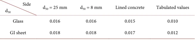
The roughness coefficient of glass and GI sheet sides as optimized for various runs are presented in Table 6.

The estimated roughness coefficients satisfy the known inequality (n2 <n3)

and are higher than the tabulated values. This establishes the credibility of the proposed model.

The optimal value of ∝ (fitting parameter) ranges from 1.42 to 1.48, which differs from the reported value i.e. 1.5. The optimal value of ∝ increases as the bed materials get finer.

Reproduction of observed profile

[image:12.595.209.541.545.623.2]

Computed GVF profiles corresponding to the optimal parameter values match quite well with corresponding observed profiles.

Table 5. Reported/Strickler’s estimated optimal estimates for bed materials.

Bed material/condition Reported/Strickler’s Estimation Optimal estimates

d50 = 20 mm 0.0247 0.032

d50 = 6 mm 0.0202 0.028

Lined concrete 0.013 - 0.015 0.027

Table 6. Reported/Strickler’s estimates and optimal estimates for sides.

Side

d50 d50 = 25 mm d50 = 8 mm Lined concrete Tabulated values

Glass 0.016 0.016 0.015 0.010

[image:12.595.211.539.657.725.2]

(13)

Variability of composite roughness

It can be observed that composite roughness reduces with increase in flow depth. Apparently because of increase in weight age of side resistance, the value of composite roughness increase.

3. Conclusions

This study was carried out to identify open channel flow parameters. Manning’s roughness coefficient and other parameters are estimated for different bed mate-rials used (d50 = 25 mm grain size, 8 mm grain size particles and Lined concrete

bed materials). Also, based on the estimated value of Manning roughness coeffi-cient and flow depths, GVF flow profile is identified.

An optimization method is applied to identify the parameters based on Man-ning formula for estimation of manMan-ning roughness coefficient and correspond-ing manncorrespond-ing roughness parameters. This estimation invokes the data of ob-served GVF profiles and such accounts for different bed materials with the flow depth.

Experimental works are done to several sets of data monitored in Hydraulics Laboratory of Civil Engineering Department. The application led to the follow-ing conclusions.

1) The GVF profile computed on the basis of estimated parameters matches quite closely with the corresponding observed profiles.

2) Strickler’s formula underestimates the roughness due to the bed material. 3) The following commonly used formula is calibrated for Manning coeffi-cient estimation

(

)

(

)

1 1

N

i i

i N

i i

n P nc

P

∝ ∝ =

∝ =

=

∑

4) The currently documented value of ∝_{is 1.5. However, the present work} reveals that it varies from 1.42 to 1.48. The value of ∝ generally decreases as the bed material gets coarser.

Conflicts of Interest

The authors declare no conflicts of interest regarding the publication of this paper.

References

[1] Atanov, G.A., Evseeva, E.G. and Meselhe, E.A. (1999) Estimation of Roughness Pro-file in Trapezoidal Open Channel. Journal of Hydraulic Engineering, 125, 309-312.

https://doi.org/10.1061/(ASCE)0733-9429(1999)125:3(309)

[2] Ayvaz, M.T. (2013) A Linked Simulation-Optimization Model for Simultaneously Estimating the Manning’s Surface Roughness Values and Their Parameter Struc-tures in Shallow Water Flows. Journal of Hydrology, 500, 183-199.

https://doi.org/10.1016/j.jhydrol.2013.07.019

(14)

https://doi.org/10.1029/WR008i004p00956

[4] Bennett, A.F. and McIntosh, P.C. (1982) Open Ocean Modeling as an Inverse Prob-lem: Tidal Theory. Journal of Physical Oceanography, 12, 1004-1018.

https://doi.org/10.1175/1520-0485(1982)012<1004:OOMAAI>2.0.CO;2

[5] Das, A. (2000) Optimal Channel Cross Section with Composite Roughness. Journal of Irrigation and Drainage Engineering, 126, 68-72.

[6] Das, S.K. and Lardner, R.W. (1991) On the Estimation of Parameters of Hydraulic Models by Assimilation of Periodic Tidal Data. Journal of Geophysical Research:

Oceans, 96, 15187-15196. https://doi.org/10.1029/91JC01318

[7] Ding, Y., Jia, Y. and Wang, S.S.M. (2004) Identification of Manning’s Roughness Coefficient in Shallow Water Flows. Journal of Hydraulic Engineering, 130, 501-510.

[8] Goldberg, D. (1989) Genetic Algorithms in Search, Optimization and Machine Learning. Addison Wesly Publishing Company, Massachusetts.

[9] Ishii, A. (2000) Parameter Identification of Manning Roughness Coefficient Using Analysis of Hydraulic Jump with Sediment Transport. Kawahara Group Research Report, Chuo University, Japan.

[10] Khatibi, R.H., Williams, J.J.R. and Wormleaton, P.R. (1997) Identification Problem of Open-Channel Friction Parameters. Journal of Hydraulic Engineering, 123, 1078-1088. https://doi.org/10.1061/(ASCE)0733-9429(1997)123:12(1078)

[11] Koza, J.R. (2010) Human-Competitive Results Produced by Genetic Programming.

Genetic Programming and Evolvable Machines, 11, 251-284.

https://doi.org/10.1007/s10710-010-9112-3

[12] Naidu, B.J., Bhallamudi, S.M. and Narasimhan, S. (1997) GVF Computation in Tree-Type Channel Networks. Journal of Hydraulic Engineering, 123, 700-708.

[13] Nguyen and Fenton (2005) Identification of Compound Channel Flow Parameters.

Advances in Hydro-Science and Engineering, 5.

[14] Ramesh, R., Datta, B., Bhallamudi, S.M. and Narayana, S. (2000) Optimal Estima-tion of Roughness in Open Channel Flows. Journal of Hydraulic Engineering, 126, 299-303. https://doi.org/10.1061/(ASCE)0733-9429(2000)126:4(299)

[15] Rodríguez-Caballero, E., Cantón, Y., Chamizo, S., et al. (2012) Effects of Biological Soil Crusts on Surface Roughness and Implications for Runoff and Erosion. Geo-morphology, 145-146, 81-89. https://doi.org/10.1016/j.geomorph.2011.12.042

[16] Sulzer, S., Rutschmann, P. and Kinzelbach, W. (2002) Flood Discharge Prediction Using Two-Dimensional Inverse Modeling. Journal of Hydraulic Engineering, 1281, 46-54. https://doi.org/10.1061/(ASCE)0733-9429(2002)128:1(46)

[17] Wasantha Lal, A.M. (1995) Calibration of Riverbed Roughness. Journal of Hydrau-lic Engineering, 121, 664-671.

[18] Wormleaton and Karmegam (1984) Parameter Optimization in Flood Routing.

Journal of Hydraulic Engineering, 110, 1799-1810.

[19] Yeh, W.W.-G. (1986) Review of Parameter Identification Procedures in Groundwa-ter Hydrology: The Inverse Problem. Water Resources Research, 22, 95-108.