Munich Personal RePEc Archive
Estimation in Non-Linear Non-Gaussian
State Space Models with Precision-Based
Methods
Chan, Joshua and Strachan, Rodney
Australian National University
2012
Online at
https://mpra.ub.uni-muenchen.de/39360/
Estimation in Non-Linear Non-Gaussian State
Space Models with Precision-Based Methods
Joshua C.C. Chan Rodney Strachany
Research School of Economics,
and Centre for Applied Macroeconomic Analysis, Australian National University
March 2012
Abstract
In recent years state space models, particularly the linear Gaussian version, have become the standard framework for analyzing macro-economic and …nancial data. However, many theoretically motivated models imply non-linear or non-Gaussian speci…cations — or both. Existing methods for estimating such models are computationally in-tensive, and often cannot be applied to models with more than a few states. Building upon recent developments in precision-based algo-rithms, we propose a general approach to estimating high-dimensional non-linear non-Gaussian state space models. The baseline algorithm approximates the conditional distribution of the states by a multivari-ate Gaussian ort density, which is then used for posterior simulation. We further develop this baseline algorithm to construct more sophis-ticated samplers with attractive properties: one based on the accept-reject Metropolis-Hastings (ARMH) algorithm, and another adaptive collapsed sampler inspired by the cross-entropy method. To illustrate the proposed approach, we investigate the e¤ect of the zero lower bound of interest rate on monetary transmission mechanism.
Corresponding author. Email: [email protected]
Keywords: integrated likelihood; accept-reject Metropolis-Hastings; cross-entropy; liquidity trap; zero lower bound
1
Introduction
State space models have proved to be very useful for modeling a wide range of processes in economics, and the linear Gaussian version has been the stan-dard speci…cation. However, economists have become increasingly aware that many processes are better represented by speci…cations that are non-linear or non-Gaussian, or both. The current preferred technique for es-timating these processes is sequential Monte Carlo methods. This paper proposes an alternative, general approach to inference in high-dimensional non-linear non-Gaussian state space models, which we believe are useful in many applications.
Building upon recent developments in precision-based algorithms for the linear Gaussian case, we present three fast sampling schemes for e¢cient simulation of the states in general state space models with multivariate ob-servations and states. The …rst algorithm, the baseline algorithm, approxi-mates the conditional distribution of the states by a multivariate Gaussian ortdensity, which is then used as a proposal density for posterior simulation using Markov chain Monte Carlo (MCMC) methods. This approximating density can also used for evaluating the integrated likelihood — the joint distribution of the observations given the model parameters but integrated over the states — via importance sampling. We then build upon this base-line approach to consider two other more e¢cient algorithms for posterior simulation. The …rst of these, our second algorithm, is the accept-reject Metropolis-Hastings (ARMH) algorithm that combines the classic accept-reject sampling and the Metropolis-Hastings algorithm. The third algorithm is a collapsed sampler used in conjunction with the cross-entropy method, where we sample the states and the model parameters jointly to reduce autocorrelations in the posterior simulator.
The speci…c framework we consider is a general state space model where the evolution of then 1vector of observations yt is governed by the
measure-ment or observation equation characterized by a generic density function
p(ytj t; ), where t is an m 1 vector of latent states and denotes the
set of model parameters. Note that the density p(ytj t; ) may depend on
previous observations yt 1; yt 2; etc. and other covariates as is the case
in the application in this paper. These observations are suppressed in the conditioning sets for notational convenience. The evolution of the states
the density function p( tj t 1; ). We note in passing that the proposed approach can be easily generalized to the case where the state equation is non-Markovian and the observationytdepends on previous states t 1; t 2;
etc.
A vast collection of models can be written in the general state space form with measurement equation p(ytj t; ) and state equation p( tj t 1; ).
Models that have proven popular among economists include time-varying parameter vector autoregressive (TVP-VAR) models, dynamic factor mod-els, stochastic volatility modmod-els, and a large class of macroeconomic models generally known as dynamic stochastic general equilibrium (DSGE) mod-els, among many others. Substantial progress has been made in the last two decades in estimating linear Gaussian state space models. For example, Kalman …lter-based algorithms include Carter and Kohn (1994), Früwirth-Schnatter (1994), de Jong and Shephard (1995) and Durbin and Koopman (2002); more recently, precision-based algorithms are proposed in Rue, Mar-tino, and Chopin (2009), Chan and Jeliazkov (2009b) and McCausland, Millera, and Pelletier (2011). E¢cient simulation algorithms also exist for certain speci…c non-linear non-Gaussian state space models, the most no-table example is the class of stochastic volatility models. Using data aug-mentation and …nite Gaussian mixtures to approximate non-Gaussian errors, Kim, Shepherd, and Chib (1998) propose a Gibbs sampler for posterior sim-ulation in a univariate stochastic volatility model. This approach is later applied to other univariate stochastic volatility models in Chib, Nardari, and Shephard (2002) and multivariate models in Cogley and Sargent (2005) and Primiceri (2005). Other successful applications of the auxiliary mixture sam-pling include state space models for Poisson counts in Frühwirth-Schnatter and Wagner (2006) and various logit models in Frühwirth-Schnatter and Frühwirth (2007). An important limitation of this approach, however, is that it is model-speci…c, and a sampler developed for one model is not gen-erally applicable to other state space models.
and resampling. For instance, particle …lters have been applied to estimat-ing non-linear DSGE models in Rubio-Ramirez and Fernandez-Villaverde (2005) and Fernandez-Villaverde and Rubio-Ramirez (2007). Despite recent advances, particle …lters are still quite computationally intensive, especially when the dimension of the states is moderately high (e.g., when m is more than 5 or 6) or when the time series is long. For Bayesian estimation, it might take tens of hours to perform a full posterior analysis. In addition, particle …lters are designed to evaluate expectations, not for e¢cient simu-lation of the states. That is, particle …lters are not designed for generating draws from the conditional density p( j ; y), where = ( 0
1; : : : ; 0T)0 and
y = (y0
1; : : : ; yT0 )0. Without samples from p( j ; y), it is more di¢cult to
design e¢cient MCMC sampling schemes to obtain posterior draws in a full Bayesian analysis. In fact, in posterior simulation with a particle …lter, it is a common practice to generate candidate draws for via a random walk sampler, and then use a particle …lter to compute the acceptance probability of the candidate draw. On the other hand, if one could generate e¢ciently from p( j ; y), one can use the machinery in the MCMC literature to de-sign an e¢cient sampling scheme to generate draws from p( j ; y). More recently, there has been work on using particle …lters to obtain candidate draws for the states (e.g., the particle Markov chain Monte Carlo methods of Andrieu, Doucet, and Holenstein, 2010). This direction looks promising, but most applications using these methods to date are limited to univariate state-space models due to computational limitations.
step. This methodology is implemented in, e.g., Shephard and Pitt (1997), Strickland et al. (2006) and Jungbacker and Koopman (2008). Departing from the obvious Gaussian approximation, McCausland (2008) recently in-troduced the HESSIAN method that provides an excellent approximation for
p( j ; y), and it results in a highly e¢cient sampling algorithm. However, the HESSIAN method requires the …rst …ve derivatives of the log-likelihood with respect to the states, which places a substantial burden on the end-user. A more severe restriction is that currently it can only be applied to univariate state space models.1
We pursue the second line of research using approximations of the condi-tional density for the states, and propose various improvements. Speci…-cally, the contributions of this paper are three-fold. In the …rst contribution we build upon the recently proposed precision-based sampler in Chan and Jeliazkov (2009b) and McCausland, Millera, and Pelletier (2011) originally developed for linear Gaussian state space models, and we present a quick method to obtain a Gaussian or a student t approximation for the condi-tional density of the statesp( j ; y). By exploiting the sparseness structure of the precision matrix forp( j ; y), the precision-based algorithm is more e¢cient than Kalman …lter-based methods in general. This feature is crucial as one needs to obtain the approximating density tens of thousands times in a full Bayesian analysis via MCMC. More importantly, the marginal cost of obtaining additional draws under the precision-based algorithm is much smaller compared to Kalman …lter-based methods. We exploit this impor-tant feature for two purposes: e¢cient simulation of the states, and evalu-ation of the integrated likelihood. We develop an accept-reject Metropolis Hastings (ARMH) algorithm for e¢cient simulation of the states. As men-tioned previously, the e¢ciency in the MH step with a Gaussian proposal can be quite low in certain settings, presumably because the Gaussian ap-proximation is not su¢ciently accurate. By using the ARMH algorithm, we construct a better approximation and consequently the acceptance rate is substantially higher compared to the baseline MH algorithm. This in-creased acceptance rate comes at a cost, however, as multiple draws from the proposal density might be required and this is why it is essential to have low marginal cost for additional draws. Next, we evaluate the integrated likelihood — an ingredient for maximum likelihood estimation and e¢cient
1One obvious way to get around this problem in multivariate-state settings is to draw
MCMC design — via importance sampling using multiple draws from the proposal density.2
The second contribution of the paper is to develop a practical way to sam-ple the model parameters and the states jointly. In performing a full Bayesian analysis, one often sequentially draws from the conditional den-sities p( jy; ) and p( jy; ). In typical situations where contains para-meters in the state equation, and are expected to be highly correlated. Consequently, the conventional sampling scheme might induce high auto-correlations for the samples, especially in high-dimensional settings. This motivates sampling and jointly by …rst drawing from p( jy) marginally of the states followed by a draw from p( jy; ). The challenge, of course, is to locate a good proposal density for , denoted asq( jy). We adopt the cross-entropy method (Rubinstein and Kroese, 2004) to obtain the optimal
q( jy) in a well-de…ned sense. Speci…cally, given a parametric family of densities G, we locate the member in G that is the closest to the marginal density p( jy) in the Kullback-Leibler divergence or the cross-entropy
dis-tance. By sampling( ; )jointly, we show via an empirical example that the
e¢ciency of the sampling scheme is substantially improved. We note that the problem of locating a good proposal density for also arises in the par-ticle …lter literature as discussed above. Hence, the proposed cross-entropy approach is useful even if the researcher chooses to use a particle …lter to evaluate the integrated likelihood instead of the algorithms discussed in this paper.
In the third contribution of the paper we demonstrate the overall approach with a topical application. We investigate the implications for transmission of monetary shocks of accounting for the zero lower bound (ZLB) on interest rates. Recent work using time-varying parameter vector autoregressive mod-els (TVP-VARs) by Cogley and Sargent (2001 and 2005), Primiceri (2005), Sims and Zha (2006) and Koop, Leon-Gonzalez and Strachan (2009) demon-strated the importance of model speci…cation for the evidence on changes in the transmission mechanism for monetary shocks. These studies considered periods of relatively high interest rates, with the exception of the period after the dot com bubble when interest rates fell as low as 1%. This latter event, and the history of Japan in the 1990s, led to an increase in interest in the e¤ect of the ZLB on the conduct of monetary policy (see, for
exam-2A further advantage of the proposed method is that it can be applied to non-Markovian
ple, Iwata and Wu, 2006, Reifschneider and Williams, 2000, and Svensson, 2003). We study the e¤ect of the ZLB on the transmission of a contrac-tionary monetary shock in a low growth, low interest rate environment. We use a TVP-VAR with a censored interest rate variable and multivariate sto-chastic volatility. Modeling volatility has proven an important requirement for accurate inference in such models (see Cogley and Sargent, 2001, 2005, Primiceri, 2005 and Sims and Zha, 2006). Our interest is in how estimates of the impulse responses to positive monetary shocks change when we allow for the ZLB.
The rest of this article is organized as follows. Section 2 …rst brie‡y discusses the precision sampler in the linear Gaussian case. In Section 3 we consider a general form of the state space model for which we propose an approximation to the conditional density for the states, an approach to estimating the integrated likelihood in this case, and the three e¢cient simulation schemes for the states. In Section 4 we apply the sampler to estimate a standard model used a number of times in the literature to investigate the evolution of the transmission of monetary shocks, but we incorporate the zero lower bound on interest rates which results in a non-linear measurement equation. Section 5 concludes and discusses various future research directions.
2
The Linear Gaussian Case
In this section we present a precision-based sampler developed indepen-dently in Chan and Jeliazkov (2009b) and McCausland, Millera, and Pel-letier (2011) for simulating the states in linear Gaussian state space models. By exploiting the sparseness structure of the precision matrix for the condi-tional density of the states, this new simulation algorithm is more e¢cient than Kalman …lter-based methods in general. In addition, the marginal cost of obtaining additional draws using the precision-based algorithm is much smaller compared to Kalman …lter-based methods, and we will take advan-tage of this fact to develop algorithms for more general model speci…cations in later sections.
Consider the following state space model:
yt=Xt t+"t; (1)
fort= 1; : : : ; T, whereyt is an n 1 vector of observations, t is an m 1
latent state vector, and the disturbance terms are jointly Gaussian:
"t t
N 0; 1
t 0
0 t1 : (3)
That is, t and t are respectively the precision matrices of"tand t. The
initial state 0 can be assumed to be a known constant or treated as a model parameter. De…ne y = (y0
1; : : : ; yT0 )0 and = ( 01; : : : ; 0T)0, and let
represent the parameters in the state space model (i.e. 0;f tg, f tg and
f tg). The covariatesfXtgare taken as given and will be suppressed in the
conditioning sets below.
From (1) and (3) it is easily seen that the joint sampling density p(yj ; ) is Gaussian. Stacking (1) over theT time periods, we have
y=X +"; " N(0; 1);
where X= 2 6 4 X1 . .. XT 3 7
5; "=
2 6 4 "1 .. . "T 3 7
5; 1 =
2 6 4 1 1 . .. 1 T 3 7 5:
A change of variable from"toy implies that
logp(yj ; )/ 1 2logj
1j 1
2(y X )
0 (y X ): (4)
It is important to realize that is a banded matrix of the form
= 2 6 4 1 . .. T 3 7 5:
For the prior distribution of , we note that the directed conditional struc-ture for p tj ; t 1 in (2) and the distributional assumption in (3) imply that the joint density for is also Gaussian. To see this, de…ne
K= 0 B B B B B @ Im
2 Im
3 Im
. .. ...
T Im
so that (2) can be written asK = + , where = 2 6 6 6 4 1 0 0 .. . 0 3 7 7 7
5 and = 2 6 6 6 4 1 2 .. . T 3 7 7 7
5 N(0;
1):
Noting thatjKj= 1, by a change of variable from to , we have
logp( j )/ 1 2logj
1j 1
2(
0)0K0 K( 0); (5)
where 0 = K 1 is the prior mean. Note that the T m T m precision
matrixK0 K is a banded matrix given by
0 B B B B B @ 0
2 2 2+ 1 02 2
2 2 03 3 3+ 2 03 3
. .. . .. . ..
T 1 T 1 0T T T + T 1 0T T
T T T
1 C C C C C A : (6) Since the likelihood functionp(yj ; ) in (4) and the priorp( j )in (5) are both linear Gaussian in , the standard update for Gaussian linear regres-sion (see, e.g. Koop, 2003, p140–141) implies that the conditional posterior
p( jy; ) / p(yj ; )p( j ) is also Gaussian. The log conditional density for the states can be written as
logp( jy; )/logp(yj ; ) + logp( j )
/ 12 0(X0 X+K0 K) 2 0(X0 y+K0 K 0) :
In other words,
( jy; ) N(b; H 1); (7)
where the precisionH and the meanb are given by
H=K0 K+X0 X; (8)
b=H 1(K0 K 0+X0 y): (9)
Since X0 X is banded, it follows that H is also banded and contains a
be obtained inO(N)operations instead of O(N3)operations for full matri-ces, where N is the dimension of the matrix. By exploiting this fact, one can sample ( jy; ) without the need to carry out an inversion to obtain
H 1 and bin (9). More speci…cally, the meanbcan be found in two steps. First, we compute the (banded) Cholesky decompositionCH ofH such that
C0
HCH =H. Second, we solve
CH0 CHb=K0 K 0+X0 y; (10)
forCHb by forward-substitution and then using the result to solve forbby
back-substitution. Similarly, to obtain a random draw fromN(b; H 1)
e¢-ciently, sampleu N(0; IT m), and solveCHx=uforxby back-substitution.
It follows thatx N(0; H 1). Adding the meanbtox, one obtains a draw
fromN(b; H 1). We summarize the above procedures in the following
algo-rithm.
Algorithm 1. E¢cient State Simulation for Linear Gaussian State Space Models
1. ComputeHin (8)and obtain its Cholesky decompositionCH such that
H=C0
HCH.
2. Solve (10) by forward- and back-substitution to obtain b.
3. Sample u N(0; IT m), and solve CHx=u for x by back-substitution.
Take =b+x, so that N(b; H 1).
By counting the number of operations, McCausland, Millera, and Pelletier (2011) show that this precision-based algorithm for simulating the states is more e¢cient than conventional Kalman-…lter based simulation methods when one draw is needed. When multiple samples are required, the mar-ginal cost of obtaining an extra draw via the precision-based algorithm is substantially less compared with the latter methods. In fact, given b and
CH, getting an additional draw from N(b; H 1)requires only (a)T m
inde-pendent standard Gaussian draws; (b) to perform a fast back-substitution to solveCHx =u for x; and (c) to add bto x. We will exploit this
3
General State Space Model
In this section we consider a general state space model where the mea-surement equation is characterized by a generic density functionp(ytj t; ),
whereas the state equation is linear Gaussian as in (2). We note that the proposed approach can be easily generalized to the case where the state equation is non-linear non-Gaussian or even non-Markovian.
3.1 Gaussian Approximation
We …rst discuss a quick method to obtain a Gaussian approximation for the conditional densityp( jy; ). This approach builds upon the precision-based algorithm outlined in Section 2. To begin, letft andGt denote respectively
the gradient and negative Hessian oflogp(ytj t; )evaluated at t=et, i.e.,
ft
@
@ tlogp(ytj t; )
t=et
; Gt
@2 @ t 0
t
logp(ytj t; )
t=et
:
Stacking these terms and de…ne the following vector and matrix:
f = 2 6 6 6 4 f1 f2 .. . fT 3 7 7 7
5; G= 2 6 6 6 4
G1 0 0
0 G2 0
..
. ... . .. ...
0 0 GT
3 7 7 7 5:
We then expand the log-likelihoodlogp(yj ; ) =PTt=1logp(ytj t; )around
e= (e01; : : : ;e0T)0 to obtain the expression
logp(yj ; ) logp(yje; ) + ( e)0f 1
2( e)
0G(
e)
= 1 2
0G 2 0(f +G
e) +c1;
(11)
where c1 is some unimportant constant independent of . Combining (11)
and the prior in (5), we have
logp( jy; )/logp(yj ; ) + logp( j ) 1
2
0(G+K0 K) 2 0(f+G
e+K0 K 0) +c2:
where c2 is some unimportant constant independent of . In other words,
the approximating distribution is Gaussian with precision H G+K0 K
and mean vectorH 1 f +Ge+K0 K 0 .
It remains to choose the pointe around which to construct the Taylor ex-pansion. One obvious choice is the posterior mode, denoted as b, which has the advantage that it can be easily obtained via the Newton-Raphson method. More speci…cally, it follows from (12) that the negative Hessian of logp( jy; ) evaluated at =e is H, while the gradient at =e is given by
@
@ logp( jy; ) =e = He+ 2(f+Ge+K
0 K 0):
Hence, we can implement the Newton-Raphson method as follows: initialize with = (1). For s= 1;2; : : :, use e= (s) in the evaluation of f,G and
H, and denote them asf( (s)),G( (s)) and H( (s)) respectively, where the
dependence on (s) is made explicit. Compute (s+1) as
(s+1) = (s)+H( (s)) 1 @
@ logp( jy; ) = (s)
=H( (s)) 1 f( (s)) +G( (s)) (s)+K0 K 0 :
(13)
If jj (s+1) (s)jj > for some pre-…xed tolerance level , then continue;
otherwise stop and set b = (s+1). Again, it is important to note that because the precision H is banded, and its Cholesky decomposition CH
can be readily obtained. Hence, (13) can be e¢ciently evaluated without inverting any high-dimensional matrix. Following the approach discussed in Section 2, we compute (s+1) as follows: given the Cholesky decomposition
CH for H( (s)), …rst solve CH0(s)x = f (s) +G( (s)) (s)+K0 K 0 for x
by forward-substitution. Then given x, solve CH (s+1) = x for (s+1) by
back-substitution. Finally, given the modeb, the negative Hessian H at b can be easily computed.
3.2 Integrated Likelihood Evaluation
The integrated likelihood p(yj ) is de…ned as the joint distribution of the data conditional on the parameter vector but integrated over the states . More explicitly,
p(yj ) =
Z
The need to evaluate the integrated likelihood e¢ciently arises in both fre-quentist and Bayesian estimation. In classical inference, one needs to max-imize the integrated likelihoodp(yj ) with respect to to obtain the max-imum likelihood estimator (MLE). In our context one has to compute the MLE numerically, and the maximization routine typically requires hundreds or even thousands of functional evaluations of p(yj ). Hence, it is crucial to be able to evaluate the integrated likelihood e¢ciently. For Bayesian es-timation, if one can evaluatep(yj ) quickly, more e¢cient samplers can be developed to obtain draws from the posterior, such as the collapsed sampler that draws and jointly in a single step which we discuss in Section 3.3.
Given the Gaussian approximation proposed in the previous section, one can estimate p(yj ) via importance sampling (see, e.g., Geweke, 1989; Kroese
et al., 2011, ch. 9). To do this, sample M independent draws 1; : : : ; M
from the proposal densityq( jy; ), and compute the Monte Carlo average
b
p(yj ) = 1
M
M
X
i=1
p(yj ; i)p( ij )
q( ijy; ) :
It is easy to see that the Monte Carlo estimator pb(yj ) is an unbiased and consistent estimator for p(yj ). In addition, if the likelihood ratio
p(yj ; )p( j )=q( jy; )or equivalentlyp( jy; )=q( jy; )is bounded for all , then the variance of the estimator is also …nite (Geweke, 1989). The proposed precision-based algorithms are especially …t for evaluating the in-tegrated likelihood via importance sampling. This is because one needs multiple draws (often hundreds or thousands) from the proposal density
q( jy; ) to compute the Monte Carlo average. As discussed earlier, one important and useful feature of the precision-based algorithms is that once we obtained the mean vector and precision matrix, additional draws can be obtained with little marginal cost.
3.3 E¢cient Simulation for the States
3.3.1 Metropolis-Hastings with Gaussian and t proposals
A simple sampling scheme is to implement a Metropolis-Hastings step with proposal densityN(b; H 1). The mode b and the negative Hessian at b of
the conditional density p( jy; ) can be computed as discussed in earlier. Moreover, a draw from the proposal can be obtained as in Algorithm 1. Us-ing a Gaussian approximation would be adequate in models where either the measurement or the state equations is Gaussian, as the resulting conditional posterior in either case has exponentially decaying tails. We summarize this basic sampling scheme as follows:
Algorithm 2. Metropolis-Hastings with the Gaussian Proposal N(b; H 1)
1. Obtain b iteratively via (13). GivenH, compute its Cholesky
decom-positionCH such thatH =CH0 CH.
2. Sample u N(0; IT m), and solve CHx=u for x by back-substitution.
Take =b+x, so that N(b; H 1).
In implementing the Metropolis-Hastings algorithm, it is often suggested that the proposal densityq( jy; )should have heavier tails than the poste-rior distributionp( jy; ), so that the likelihood ratio p( jy; )=q( jy; ) is bounded. This is important because a bounded likelihood ratio ensures the geometric ergodicity of the Markov chain (Roberts and Rosenthal, 2004). In the context of estimating the integrated likelihood, this guarantees the esti-mator has …nite variance. Thus, one concern of using a Gaussian proposal is that it has exponentially decaying tails, and consequently, the likelihood ratio might not be bounded. This motivates using a proposal density with heavier tails, such at distribution. We note that one can easily modify the above Gaussian approximation to obtain atproposal density instead. More explicitly, consider the tproposal q( jy; ) t( ;b; H 1) with degree
of freedom parameter , location vectorb and scale matrixH 1. Note that
sampling from t( ;b; H 1) involves only T m iid standard Gaussian draws
and a draw from theGamma( =2; =2) distribution. We summarize the
al-gorithm as follows:
Algorithm 3. Metropolis-Hastings with the t proposal t( ;b; H 1)
1. Given the posterior modeband negative HessianH, obtain the Cholesky
2. Sample u N(0; IT m) and r Gamma( =2; =2). Then v u=pr t( ;0; IT m).
3. Solve CHx =v for x by back-substitution and take =b+x, so that
t( ;b; H 1).
3.3.2 Accept-Reject Metropolis-Hastings
As its name suggests, the accept-reject Metropolis-Hastings (ARMH) algo-rithm (Tierney, 1994; Chib and Greenberg, 1995) is an MCMC sampling procedure that combines classic accept-reject sampling with the Metropolis-Hastings algorithm. In the our setting the target density is the condi-tional density of the states p( jy; ) / p(yj ; )p( j ). Suppose we have a proposal densityq( jy; ) from which we generate candidate draws (e.g.
q( jy; )can be the Gaussian ortdensity discussed in the previous section). In the classic accept-reject sampling a key requirement is that there exists a constantc such that
p(yj ; )p( j )6cq( jy; ); (15) for all in the support of p( jy; ). When is a high-dimensional vector, as in the present case, such a constant c, if it exists, is usually di¢cult to obtain. To make matters worse, the target density p( jy; ) depends on other model parameters that are revised at every iteration. Finding a new value of c for each new set of parameters might signi…cantly increase the computational costs. The ARMH relaxes the domination condition (15) such that when it is not satis…ed for some , we resort to the MH algorithm. To present the algorithm, it is convenient to …rst de…ne the set
D=f :p(yj ; )p( j )6cq( jy; )g;
and letDc denote its complement. Then the ARMH algorithm proceeds as
follows:
Algorithm 4. Accept-Reject Metropolis-Hastings with Gaussian or t pro-posal
1. AR step: Generate a draw q( jy; ), where q( jy; ) is the
probability
AR( jy; ) = min 1;
p(yj ; )p( j )
cq( jy; ) :
Continue the above process until a draw is accepted.
2. MH-step: Given the current draw and the proposal
(a) if 2 D, set M H( ; jy; ) = 1;
(b) if 2 Dc and 2 D, set
M H( ; jy; ) =
cq( jy; )
p(yj ; )p( j );
(c) if 2 Dc and 2 Dc, set
M H( ; jy; ) = min 1;
p(yj ; )p( j )q( jy; )
p(yj ; )p( j )q( jy; ) :
Return with probability M H( ; jy; ); otherwise return .
As shown in Chib and Greenberg (1995), the draws produced at the com-pletion of the AR step have the density
qAR( jy; ) =d 1 AR( jy; )q( jy; );
where dis the normalizing constant (which needs not be known for imple-menting the algorithm). In other words, one might view the AR step as a means to sample from the density qAR( jy; ). By adjusting the original
proposal densityq( jy; )by the function AR( jy; ), a better
approxima-tion of the target density is achieved. In fact, we have
qAR( jy; ) = pq((yj ; )p( j )=cd; 2 D;
jy; )=d; 2 Dc;
i.e., the new proposal density coincides with the target density on the setD (albeit with di¤erent normalizing constants), whereas on Dc the new
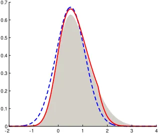
the true density for values less than 1.6, then di¤ers above this point but still …ts better than the Gaussian density. The better approximation, of course, comes at a cost, because multiple draws from the proposal density
q( jy; ) might be required in the AR step. This is where the precision-based method (as in Algorithms 2 or 3) comes in. As we have emphasized before, the marginal cost of generating additional draws using the precision-based method is low, and is substantially lower than generating candidate draws via Kalman …lter-based algorithms. In fact, as demonstrated in the application, the gain in e¢ciency under the ARMH sampling scheme more than justi…es its additional cost compared to a plain MH step.
-2 -1 0 1 2 3 4
[image:19.612.226.385.286.425.2]0 0.1 0.2 0.3 0.4 0.5 0.6 0.7
Figure 1: Illustration of the two approximations for a skew normal distri-bution (shaded): Gaussian (dotted line) and the same Gaussian with AR adjustment (solid line).
Chib and Jeliazkov (2005) present a practical way to select the constant c
and the trade-o¤ in such a choice which we outline here. Notice that if a biggercis chosen, then the set Dis larger and we are more likely to accept the candidate . The cost, on the other hand, of selecting a larger c is that more draws from q( jy; ) are required in the AR step. A practical way to strike a balance between these two con‡icting considerations is to set c=rp(yjb; )p(bj )=q(bjy; ), where bis the mode of the conditional densityp( jy; )andr is, say, between 1 and 5. Such a choice would ensure that c is su¢ciently small to reduce the required number of draws from
3.3.3 Collapsed Sampling with the Cross-entropy Method
We have so far discussed two sampling schemes for e¢cient simulation from the conditional density p( jy; ): the MH and the ARMH algorithms with either a Gaussian or atproposal. In performing a full Bayesian analysis, one often sequentially draws fromp( jy; )followed by sampling fromp( jy; ). In typical situations where contains parameters in the state equation, and are expected to be highly correlated. Consequently, the conventional sampling scheme might induce high autocorrelation and slow mixing in the Markov chain, especially in high-dimensional settings. For this reason, we seek to sample ( ; ) jointly by …rst drawing fromp( jy) marginally of the states followed by a draw from p( jy; ), where the latter step can be accomplished by either the MH or ARMH algorithm previously discussed. To sample fromp( jy), we again implement a MH step: we …rst generate a candidate draw from the proposal density g( ), then we decide whether to accept or not according to the acceptance probability. Hence, we need two ingredients: (1) a quick routine to evaluate the integrated likelihood
p(yj ), which arises in computing the acceptance probability; and (2) a good proposal densityg( )for generating candidate draws for the MH step.
The …rst ingredient, an e¢cient method to evaluate the integrated likeli-hood, is provided by the importance sampling estimator pb(yj ) discussed in Section 3.2. And this in turn gives us an estimator for the acceptance probability
( jy) = min 1;p(yj )p( )g( ) p(yj )p( )g( ) :
One might raise the concern that the simulation error may a¤ect the conver-gence properties of the Markov chain, as the candidate draws are accepted or rejected according to estimated acceptance probabilities rather than the actual values. However, since the importance sampling estimatorpb(yj ) is unbiased, the results in Andrieu, Berthelsen, Doucet, and Roberts (2007) and Flury and Shephard (2008) show that the stationary distribution of the constructed Markov chain is the posterior distribution as desired.
We adopt the so-called cross-entropy adaptive independence sampler intro-duced in Keith, Kroese, and Sofronov (2008). Speci…cally, the proposal den-sity is chosen such that theKullback-Leibler divergence, or thecross-entropy
(CE)distance between the proposal density and the target (the posterior
density) is minimal, where the CE distance between the densitiesg1 and g2
is de…ned as:
D(g1; g2) =
Z
g1(x) log
g1(x)
g2(x)
dx:
LetG be a parametric family of densities g( ; v) indexed by the parameter vectorv. Minimizing the CE distance is equivalent to …nding
vce = argmax v
Z
p( jy) logg( ;v)d :
As in the CE method (Rubinstein and Kroese, 2004; Kroese, Taimre, and Botev, 2011, ch. 13), we can estimate the optimal solution vce by
b
vce = argmax v
1
N
N
X
i=1
logg( i;v); (16)
where 1; : : : ; N are draws from the marginal posterior densityp( jy). The
solution to the maximization problem in (16) is typically easy to obtain; in fact, analytic solutions are often available. On the other hand, …nding
b
vce requires a pre-run to obtain a small sample from p( jy). This can be
achieved by sequentially drawing fromp( jy; ) and p( jy; ), as discussed in the previous section. It is important to note that although the sample obtained in this pre-run may exhibit slow mixing, we only use it to obtain the proposal density, and thus it has little adverse e¤ect on the main collapsed sampler. Once we …nd vbce, we then use the proposal density g( ;bvce) to
implement the independence-chain MH step. We discuss in more details the implementation in Appendix B.
4
Application
lower bound (ZLB) on interest rates. With time varying parameters, incor-porating the lower bound on interest rates introduces a non-linearity in the states into the measurement equation. Recent work using time-varying pa-rameter vector autoregressive models (TVP-VARs) on changes in the trans-mission mechanism for monetary policy shocks (see for example, Cogley and Sargent, 2001, 2005, Primiceri, 2005, Sims and Zha, 2006, and Koop, Leon-Gonzalez and Strachan, 2009) has ignored the lower bound on interest rates. Not accounting for the ZLB is reasonable when interest rates are relatively high and far from zero. However, episodes of low interest rates have occurred often in recent history including, as examples, in the US just after the dot com bubble of 2001, during the 1990s in Japan, or since 2009 in much of the developed world. The prevalence of low interest rates suggests it is im-portant to know whether transmission of monetary shocks is a¤ected and, if so, to understand how the transmission mechanism is a¤ected. Our focus is upon the e¤ect of a contractionary monetary shock when interest rates are on the ZLB. Such a situation might arise for the US if several rating agencies were to downgrade the rating of US government debt and creditors then began to demand a premium to compensate for the risk of default, or if the cost of funds to banks increased independently of moves in the Federal Funds rate inducing an e¤ective, unintended tightening of monetary policy.3
4.1 The Model
The framework we consider is the following time-varying parameter vector autoregressive (TVP-VAR) model withl lags:
yt= t+A1tyt 1+ +Altyt l+ t; t N(0; t1);
where t is ann 1 vector of time-varying intercepts,At1; : : : ; Atl aren n
matrices of VAR lag coe¢cients at timet, and t1is a time-varying precision matrix. For the purpose of estimation, we write the VAR system in the form of seemingly unrelated regressions:
yt=xt t+ t; t N(0; t1); (17) 3This e¤ect was observed in February 2012 in Australia when, after the central bank
kept its rate unchanged, all banks increased their lending rates in response to increased costs of wholesale funding costs.
where xt = In [1; y0t 1; : : : ; y0t l] and t = vec([ t : A1t : : Alt]0) is
a k 1 vector of VAR coe¢cients with k = n2l+n. To model the
time-varying precision matrix t, we follow the approach proposed in Primiceri
(2005) by …rst factoring the precision matrix as t=L0tDt1Lt, where Dt=
diag(eh1t; : : : ;ehnt)is a diagonal matrix, andL
tis a lower triangular matrix
with ones on the main diagonal, i.e.,
Dt=
0 B B B @
eh1t 0 0 0 eh2t 0
..
. ... . .. ... 0 0 ehnt
1 C C C
A; Lt= 0 B B B B B B @
1 0 0 0
a21;t 1 0 0
a31;t a32;t 1 ...
..
. ... ... . .. ...
an1;t an2;t an(n 1);t 1
1 C C C C C C A :
This decomposition has been employed in various applications, especially in the context of e¢cient estimation of covariance matrices (Pourahmadi, 1999, 2000, Smith and Kohn, 2002, Chan and Jeliazkov, 2009a, among others). In the setting of VAR models with time-varying volatility, this approach is …rst considered in Cogley and Sargent (2005). For notational convenience, we letht= (h1t; : : : ; hnt)0 and hi = (hi1; : : : ; hiT)0. That is,ht is then 1
vector obtained by stackinghitby the …rst subscript, whereashi is theT 1
vector obtained by stackinghitby the second subscript. The log-volatilities
htevolve according to the state equation
ht=ht 1+ t; t N(0; h1); (18)
fort = 2; : : : ; T; where h =diag(!h1; : : : ; !hn) is a diagonal matrix. The
process is initialized withh1 N(0; Vh 1)for some known diagonal precision
matrix Vh. Let at denote the free elements in Lt ordered by rows, i.e.,
at at = (a21;t; a31;t; a32;t; : : : ; an(n 1);t)0, so that at is an m 1 vector of
parameters where m = n(n 1)=2. The evolution of at is modeled as a
random walk
at=at 1+ t; t N(0; a1); (19)
fort= 2; : : : ; T; where a=diag(!a1; : : : ; !am) is a diagonal precision
ma-trix. The process is initialized witha1 N(0; Va 1)for some known diagonal
precision matrix Va. In what follows we use these two parameterizations,
namely, t and (ht; at), interchangeably. To complete the speci…cation of
the model, it remains to specify the evolution of the VAR coe¢cients t. We follow the standard approach of modeling the VAR coe¢cients t as a random walk process:
for t = 2; : : : ; T; where = diag(! 1; : : : ; ! k) is a diagonal precision
matrix. The process is initialized with 1 N(0; V 1) for some known
precision matrixV .
After presenting the basic setup of a TVP-VAR model with stochastic volatility, we now wish to impose the restriction that the nominal inter-est rate is always non-negative. For this purpose, arrange the data yt so
thaty1t, the …rst element of yt, is the nominal interest rate, and let x1t be
the …rst row of xt. We assume that y1t > 0. Consequently, given t and t, yt follows a multivariate Gaussian distribution with the …rst element
restricted to be positive. To derive the likelihood function, …rst note that since onlyy1tis constrained while other elements ofytare not, the marginal
distribution of y1t is a univariate Gaussian variable truncated below at 0.
In fact, it can be easily shown that
(y1tj t; t) N(x1t t;eh1t)1l(y1t>0):
It follows that given t and t, we have
P(y1t>0j t; t) = 1 x1t t=e
1 2h1t
= x1t te
1 2h1t
;
where ( )denotes the standard Gaussian cumulative distribution function. Letting y = (y0
1; : : : ; yT0 )0, = ( 01; : : : ; 0T)0 and = ( 1; : : : ; T), the
log-likelihood function is thus
logp(yj ; ) =
T
X
t=1
logp(ytj t; t); (21)
where
p(ytj t; t)/ 1
2logj
1
t j
1
2(yt xt t)
0
t(yt xt t) log x1t te
1 2h1t
:
4.2 Prior and Estimation
Speci…cally, the elements of! ,!hand!afollow independently Gamma
dis-tributions: ! i Gamma(r i; s i) fori = 1; : : : ; k, !hi Gamma(rhi; shi);
fori= 1; : : : ; n;and!ai Gamma(rai; sai);fori= 1; : : : ; m. For later
refer-ence, we stackh= (h0
1; : : : ; h0T)0 anda= (a01; : : : ; a0T)0, and let denote the
set of parameters except the latent states , hand a, i.e., = (! ; !h; !a).
In what follows, we brie‡y discuss the implementation of the three samplers; we refer the readers to Appendices A and B for more details. The …rst sampling scheme is the baseline Metropolis-Hastings sampler that involves sequentially drawing from:
a. p( jy; h; a; ) via an MH step; b. p(hjy; ; a; ) via an MH step; c. p(ajy; ; h; ) via a Gibbs step; d. p( jy; ; h; a) via a Gibbs step.
To e¢ciently sample the states in the non-linear state space model (20) and (21), we consider implementing an independence-chain MH step by ap-proximating the conditional distribution p( jy; h; a; ) via a Gaussian dis-tribution as discussed in Section 3.1. The next step is to sample from the conditional distribution p(hjy; ; a; ). Recall that hit is the i-th diagonal
element in Dt, ht = (h1t; : : : ; hnt)0 and hi = (hi1; : : : ; hiT)0. Note that
we are able to write logp(hjy; a; ; ) = Pni=1logp(hi jy; a; ; ): What
this means is that to obtain a draw from p(hjy; a; ; ), we can instead sample fromp(hi jy; a; ; )sequentially without adversely a¤ecting the
ef-…ciency of the sampler. Now, a draw from p(hi jy; a; ; ) can be obtained
via an independence-chain Metropolis-Hastings step with a Gaussian pro-posal density; more details are given in Appendix A. Thirdly, it can be easily shown that p(ajy; ; h; ) is a Gaussian distribution (see, e.g. Prim-iceri, 2005), and a draw from which can be obtained using Algorithm 1. Finally, p( jy; ; h; a) is a product of Gamma densities, and a draw from which is standard (see Koop, 2003, p. 61-62).
a. p(! jy; h; a) marginally via an MH step, followed by p( jy; h; a; ) via an ARMH step;
b. p(!hjy; ; a) marginally via an MH step, followed by p(hjy; ; a; )
via an ARMH step;
c. p(!ajy; ; h) marginally via an MH step, followed by p(ajy; ; h; )
via a Gibb step.
The details for the collapsed sampler are given in Appendix B.
4.3 Empirical Results
We now present empirical results based on a set of U.S. macroeconomic variables commonly used in the study of the evolution of monetary policy transmission. We have an interest rate to capture e¤ects of monetary con-ditions, a real growth rate variable to capture the state of the economy, and in‡ation. The dataset is obtained from the U.S. Federal Reserve Bank at St. Louis website that consists quarterly observations from 1947Q1 to the 2011Q2 on the following n = 3 U.S. macroeconomic series: U.S. 3-month Treasury bill rate, CPI in‡ation rate, and real GDP growth. Both the CPI in‡ation rate and real GDP growth are computed via the formula 400(log(zt) log(zt 1)), where zt is the original quarterly CPI or GDP
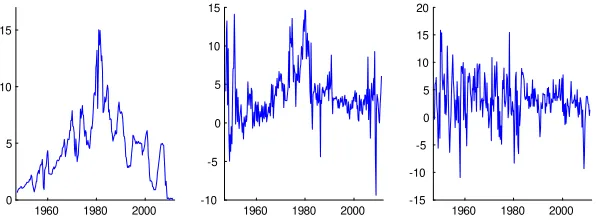
…g-ures. The inclusion of the interest rate variable which is bounded below at zero, provides a useful example to demonstrate our methods. The plot the evolution of the interest rate, given in Figure 2, shows that since the start of the quantitative easing in late 2008, the 3-month Tbill rate has become essentially zero.
1960 1980 2000 0
5 10 15
1960 1980 2000 -10
-5 0 5 10 15
1960 1980 2000 -15
[image:27.612.166.464.136.246.2]-10 -5 0 5 10 15 20
Figure 2: The U.S. 3-month Tbill rate (left), CPI in‡ation rate (middle), and GDP growth rate (right) from 1947 Q1 to 2011 Q2.
unrestricted model can be estimated using the standard outlined in Section 2.
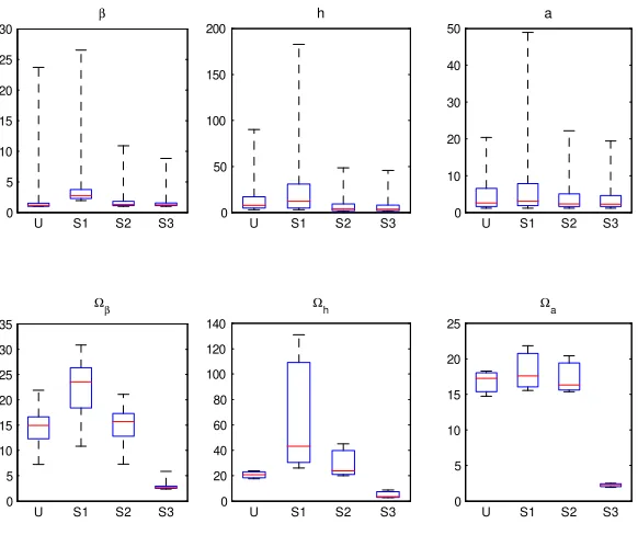
One popular measure of MCMC e¢ciency is the ine¢ciency factor, de…ned as:
1 + 2
J
X
j=1
j;
where j is the sample autocorrelation at lag length j, and J is chosen large enough so that the autocorrelation tapers o¤. This statistic approx-imates the ratio of the numerical variance of the posterior mean from the MCMC output relative to that from hypothetical iid draws. As the poste-rior draws from the Markov chain become less serially correlated, the ratio will approach the ideal minimum value of 1. In the presence of ine¢ciency due to serial correlation in the draws, the ratio will be larger than 1. Fig-ure 3 presents the boxplots of the ine¢ciency factors for the four sampling schemes.
Remember that the unrestricted model is linear Gaussian and can be esti-mated via standard Gibbs sampler. In contrast, the restricted model that incorporates the ZLB is non-linear, and the conditional densities of the states are non-standard. Since the proposed samplers need to approximate these conditional densities, we would generally expect that they would not per-form as well compared to the standard Gibbs sampler used to estimate the
unrestricted model. As evidenced by the plots in Figure 3, the proposed
0 5 10 15 20 25 30
U S1 S2 S3
β 0 50 100 150 200
U S1 S2 S3
h 0 10 20 30 40 50
U S1 S2 S3
a 0 5 10 15 20 25 30 35
U S1 S2 S3
Ωβ 0 20 40 60 80 100 120 140
U S1 S2 S3
Ωh 0 5 10 15 20 25
U S1 S2 S3
[image:28.612.165.456.141.385.2]Ωa
Figure 3: Boxplots of the ine¢ciency factors for the unrestricted linear Gaussian model (U), and the three sampling schemes: MH (S1), ARMH (S2) and the collapsed sampler (S3). The central mark of each box is the median, the edges of the box are the 25th and 75th percentiles, and the whiskers extend to the maximum and minimum.
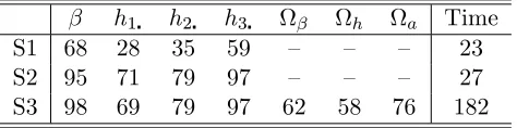
Table 1: Acceptance rate (in %) and the computing time (in minutes) of the three sampling schemes: MH (S1), ARMH (S2) and the collapsed sampler with CE (S3).
h1 h2 h3 h a Time
S1 68 28 35 59 – – – 23
S2 95 71 79 97 – – – 27
S3 98 69 79 97 62 58 76 182
is as good as S3 for the states, but it is worse than S3 for the estimation of the state precisions.
In Table 1 we present the acceptance rates of draws from candidates, as well as the computation time for obtaining 50,000 draws. On the whole the three samplers are relatively fast and have reasonable acceptance rates. These results are more signi…cant given our high-dimensional model: has more than 3,000 elements andh has more than 750. To compare among the three sampling schemes, we see that although S1 is relatively fast, it can have low acceptance rates particularly for the log volatilities. By contrast, S2 has higher acceptance rates at the expense of only a little more compu-tation time. Although S3 is more e¢cient relative to S2 in terms of lower ine¢ciency factors, its computation time is almost seven times compared to that of S2. For our model and dataset, it would seem that S2 is the best among the three.
We now present empirical results for the restricted model estimated using the ARMH sampler (S2). For comparison, we also report the corresponding results for the unrestricted model. This comparison is provided to demon-strate the implications for inference of neglecting the restriction of the ZLB. We begin with a discussion of the implications of the restriction for parame-ter estimation and then show the e¤ect on impulse responses of not correctly accounting for the ZLB. These di¤erences are signi…cant and justify the new estimation methods presented in this paper.
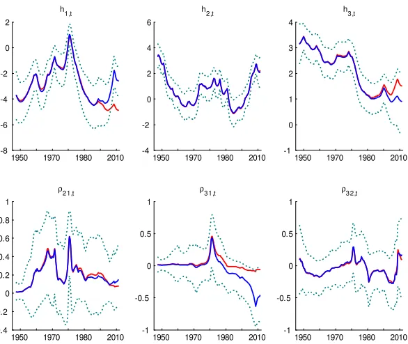
The e¤ect of neglecting the ZLB restriction shows up in all blocks of pa-rameters: the variances; the correlations; and mean equation coe¢cients. Figure 4 shows the estimated log-volatilities and correlations for the re-stricted model and the unrere-stricted model. The …gure for the log-volatilities of the monetary shock, h1;t, shows that ignoring the restriction would lead
1950 1970 1980 2010 -8 -6 -4 -2 0 2 h 1,t
1950 1970 1980 2010 -0.4 -0.2 0 0.2 0.4 0.6 0.8 1 ρ21,t
1950 1970 1980 2010 -4 -2 0 2 4 6 h 2,t
1950 1970 1980 2010 -1 -0.5 0 0.5 1 ρ31,t
1950 1970 1980 2010 -1 0 1 2 3 4 h 3,t
[image:30.612.164.457.136.383.2]1950 1970 1980 2010 -1 -0.5 0 0.5 1 ρ32,t
Figure 4: Evolution of the log-volatilities and correlations. The solid red line is the estimated posterior mean under the unrestricted model. The solid blue line is the estimated posterior mean and the dotted green lines are the 5%-tile and 95%-tile, respectively, under the model with the inequality restrictions imposed.
The monetary shock volatility is much higher than the unrestricted model suggests. Similarly the volatility of real activity,h3;t, is over estimated when
the ZLB is ignored. The volatility and correlations of the nominal variable shock does not show much in‡uence from the ZLB. However, the correlation of the error from the interest rate equation with the error from the growth equation is strongly a¤ected, this correlation would be estimated as being near zero rather than very negative. This e¤ect has important implications for the impulse responses.
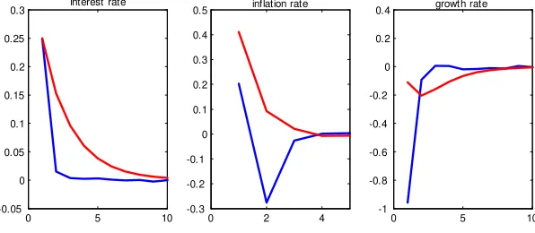
im-pulse responses as the di¤erences in forecasts. However, due to the non-linear form of the model, these impulses are not the standard ones derived from the VMA representation in linear models. We forecast the variables using the parameter values at 2011 Q2, assuming the parameters cease evolving, but taking into account the ZLB into these forecasts. We then forecast again, but increase the error in the interest rate equation, the monetary shock, by 0.25%. Our impulse responses are the di¤erences between these two fore-casts. We see that there is a faster response of interest rates to the monetary shock, but the form of the response is similar.
0 5 10
-0.05 0 0.05 0.1 0.15 0.2 0.25
0.3 interest rate
0 2 4
-0.3 -0.2 -0.1 0 0.1 0.2 0.3 0.4
0.5 inflation rate
0 5 10
-1 -0.8 -0.6 -0.4 -0.2 0 0.2
[image:31.612.157.455.269.399.2]0.4 growth rate
Figure 5: Impulse response of a 0.25% increase in interest rate under the unrestricted model (red solid line) and the model with the inequality restric-tions imposed (blue solid line).
unanticipated monetary shocks.
5
Concluding Remarks and Further Research
In this paper we have proposed a new approach to e¢ciently estimate high-dimensional non-linear non-Gaussian state space models. Due to the general applicability of the proposed approach, it will prove useful in a wide range of applications. We extend the recently developed precision-based samplers (Chan and Jeliazkov, 2009b and McCausland, Millera, and Pelletier, 2011) and sparse matrix procedures to build fast, e¢cient samplers for these non-linear models. We develop a practical way to sample the model parameters and the states jointly to circumvent the problem of high autocorrelations in high-dimensional settings. This approach uses the cross-entropy method (Rubinstein and Kroese, 2004) to obtain the optimal candidate densities
q( jy). We show via an empirical example that the e¢ciency of the sampling scheme is substantially improved by drawing ( ; y) jointly. Three samplers are presented each with virtues in di¤erent circumstances. Finally, we apply these techniques in a TVP-VAR in which one of the variables is restricted to be strictly positive. Using this framework, we investigate the implications for transmission of monetary shocks of accounting for the zero lower bound (ZLB) on interest rates.
Another advantage of the proposed method is that it can be applied to non-Markovian state equations, which arise in, e.g., various non-linear DSGE models, and they are more di¢cult to handle under other approaches. There-fore in future work we will apply this approach to the estimation of non-linear DSGE models. Another direction will be in models with measurement equations that involving more than current, past or even future states.
Appendix A: E¢cient Simulation of
and
h
the decomposition t=L0tDt1Lt, where
Dt=
0 B B B @
eh1t 0 0 0 eh2t 0
..
. ... . .. ... 0 0 ehnt
1 C C C
A; Lt= 0 B B B B B B @
1 0 0 0
a21;t 1 0 0
a31;t a32;t 1 ...
..
. ... ... . .. ...
an1;t an2;t an(n 1);t 1
1 C C C C C C A :
Recall that hit is the i-th diagonal element in Dt, ht = (h1t; : : : ; hnt)0 and
hi = (hi1; : : : ; hiT)0. That is,htis then 1vector obtained by stackinghit
by the …rst subscript, whereashi is theT 1vector obtained by stackinghit
by the second subscript. Also,atdenotes the free elements inLt ordered by
rows, i.e., at = (a21;t; a31;t; a32;t; : : : ; an(n 1);t)0. In what follows we use the
two parameterizations tand(ht; at)interchangeably. Then the log-density
foryt given( t; t)is
logp(ytj t; t)/
1
2(yt xt t)
0
t(yt xt t) log ( t);
where t=x1t te
1
2h1t:Using the notation in Section 3.1, we have
ft @
@ tlogp(ytj t; t)
t=et
; Gt @
2
@ t 0tlogp(ytj t; t)
t=et
;
where
@
@ tlogp(ytj t; t) =x
0
t t(yt xt t) ( t)
( t)
e 12h1t
x01t;
@2
@ t 0tlogp(ytj t; t) = x
0
t txt+ ( t)
( t)
e h1t
t+ ( t)
( t)
x01tx1t;
where ( ) and ( )denote the standard Gaussian probability density func-tion and cumulative distribufunc-tion funcfunc-tion respectively. Givenft andGt, we
can then use the Gaussian ortapproximations in Section 3.1 as a proposal density.
We now discuss sampling from the conditional density p(hjy; a; ; ). We …rst show that
logp(hjy; a; ; ) =
n
X
i=1
Put di¤erently, to obtain a draw fromp(hjy; a; ; ), we can instead sample from p(hi jy; a; ; ) sequentially without adversely a¤ecting the e¢ciency
of the sampler. To this end, decompose t = L0tDt 1Lt as before. Since
logj tj = logjDtj = Pni=1hit and 2t;11 = eh1t, it follows that the
log-likelihood is given by
logp(yj ; h; a; )/
T X t=1 " 1 2 n X i=1 hit 1 2(Lt t)
0D 1
t Lt t log e h1t=2x1t t
# ; = T X t=1 " 1 2 n X i=1
hit 1
2
n
X
i=1
e hit
s2it log e h1t=2
x1t t
# ;
(22)
where t = yt xt t and s2it is the i-th diagonal element of (Lt t)(Lt t)0.
On the other hand, the state equation (18) implies that each hi follows
independently a Gaussian distribution. In fact, we have
hit=hi;t 1+ it; it N(0; !hi): (23)
Hence, it follows from (22) and (23) that hi; i= 1; : : : ; n are conditionally
independent given the data and other parameters.
We note that although one can apply the auxiliary variable approach in Kim, Shepherd, and Chib (1998) to sample from p(hi jy; a; ; ) for i =
2; : : : ; n, it cannot be used to draw from p(h1 jy; a; ; ) due to the extra
termlog e h1t=2x
1t t in the log-likelihood (22) that depends on t.
In-stead, we sample eachhi sequentially via an independence-chain
Metropolis-Hastings step. As before, we …rst derive an expression for a second or-der Taylor expansion of the log-likelihood (22) around the posterior mode
bhi = (bhi1; : : : ;bhiT)0. De…ne t=e h1t=2x1t t
qit =
@ @hit
logp(yj ; h; a; )
hit=bhit
; rit=
@2 @h2
it
logp(yj ; h; a; )
hit=bhit
;
qi = (qi1; : : : ; qiT)0 and Ri =diag(ri1; : : : ; riT), where
@ @hit
logp(yj ; h; a; ) = 1 2 e
hits2
it 1 + t
( t)
( t)1l(i= 1) ; and
@2
@h2itlogp(yj ; h; ) =
1 2e
hits2
it+
1 4 t
( t) ( t)
2
t + t
( t)
If we expand the log-likelihood (22) around the modebhi, we have
logp(yj ; h; a; ) 1 2
h b
h0iRibhi 2bh0i(qi+Ribhi)
i
+c3;
wherec3 is some unimportant constant independent ofbhi. We consider the
proposal densityN(bhi;(qi+Ribhi) 1), and everything follows as before.
Appendix B: Collapsed Sampler with the
Cross-Entropy Method
In this appendix we provide the details on the collapsed sampler used in the third sampling scheme. In a nutshell, we …rst use a small posterior sample from a pre-run and the cross-entropy method to locate an optimal proposal density within a given parametric family. Then given a candidate draw from the proposal, we implement a Metropolis-Hastings step to decide whether or not to accept the candidate, where the acceptance probability is computed using the importance sampling estimator for the integrated likelihood proposed in Section 3.2. We focus on discussing the approximation to p(! jy; h; a), where ! = (! 1; : : : ; ! k)0. The approximations to the
other two marginal densities follow similarly. Recall that the elements of!
have an independent gamma prior: ! i Gamma(r i; s i) for i= 1; : : : ; k.
Therefore, a natural parametric family within which to locate the proposal density is the gamma family:
G=
( k Y
i=1
fG(! i;c i; d i)
) ;
wherefG( ;c; d) is the density ofGamma(c; d). Given theR posterior draws
f!(j1); : : : ; !(jk)g,j= 1; : : : ; R, we solve the CE optimization problem in (16) to obtainbvce = (bc 1;db1; : : : ;bc k;dbk):Speci…cally, the optimal CE reference
parameter vectorbvce can be obtained as follows. First note thatdbi can be
solved analytically givenc i:
b d i =
Rc i
PR j=1!
(j)
i
:
Now by substitutingd i =dbi into the densityfG( ;c i; d i); bc i can be
method). Hence, we can obtain (bc 1;db1; : : : ;bc k;dbk) easily. Finally, the
proposal density is
f (! ) =
k
Y
i=1
fG(! i;bc i;dbi);
which is the member withinG that is the closest in cross-entropy divergence to the marginal density p(! jy; h; a).
References
Andrieu, C. , K. K. Berthelsen, A. Doucet, and G. O. Roberts. The expected auxiliary variable method for Monte Carlo simulation. Technical report, 2007.
Andrieu, C., A. Doucet and R. Holenstein. Particle Markov chain Monte Carlo methods. Journal of the Royal Statistical Society Series B, 72:269– 342, 2010.
Carter, C. K., and R. Kohn. On Gibbs sampling for state space models. Biometrika, 81:541–553, 1994.
Chan, J. C. C., and I. Jeliazkov. MCMC estimation of restricted covariance matrix. Journal of Computational and Graphical Statistics, 18:457–480, 2009a.
Chan, J. C. C., and I. Jeliazkov. E¢cient simulation and integrated likeli-hood estimation in state space models. International Journal of Mathemat-ical Modeling and NumerMathemat-ical Optimisation, 1:101–120, 2009b.
Chib, S., and E. Greenberg. Understanding the Metropolis-Hastings algo-rithm. The American Statistician, 49(4):327–335, 1995.
Chib, S., and I. Jeliazkov. Accept-reject Metropolis-Hastings sampling and marginal likelihood estimation. Statistica Neerlandica, 59:30–44, 2005.
Cogley, T. and T. J. Sargent. Evolving post-World War II in‡ation
dynam-ics,NBER Macroeconomic Annual, 16, 331-373, 2001.
Cogley, T., and T. J. Sargent. Drifts and volatilities: monetary policies and outcomes in the post WWII US. Review of Economic Dynamics, 8(2):262 – 302, 2005.
de Jong, P., and N. Shephard. The simulation smoother for time series models. Biometrika, 82:339–350, 1995.
Doucet, A., and A. M. Johansen. A tutorial on particle …ltering and smooth-ing: Fifteen years later. In D. Crisan and B. Rozovskii, editors, The Oxford Handbook of Nonlinear Filtering. Oxford University Press, Oxford, 2011.
Doucet, A., N. De Freitas, and N.J. Gordon, editors. Sequential Monte Carlo Methods in Practice. Springer, New York, 2001.
Durbin, J., and S. J. Koopman. Monte Carlo maximum likelihood estima-tion for non-Gaussian state space models. Biometrika, 84:669–684, 1997.
Durbin, J., and S. J. Koopman. A simple and e¢cient simulation smoother for state space time series analysis. Biometrika, 89:603–615, 2002.
Fernandez-Villaverde, J., and J. F. Rubio-Ramirez. Estimating macro-economic models: A likelihood approach. Review of Economic Studies, 74(4):1059–1087, 2007.
Flury, T., and N. Shephard. Bayesian inference based only on simulated likelihood: particle …lter analysis of dynamic economic models. Economics SeriesWorking Papers 413, University of Oxford, Department of Economics, 2008.
Früwirth-Schnatter, S. Data augmentation and dynamic linear models. Jour-nal of Time Series AJour-nalysis, 15:183–202, 1994.
Frühwirth-Schnatter, S., and R. Frühwirth. Auxiliary mixture sampling with applications to logistic models. Computational Statistics & Data Analy-sis, 51(7):3509–3528, 2007.
Geweke, J. Bayesian inference in econometric models using Monte Carlo integration. Econometrica, 57 (6):1317–1339, 1989.
Iwata, S. and S. Wu. Estimating monetary policy e¤ects when interest rates are close to zero. Journal of Monetary Economics, Elsevier, vol. 53(7), pages 1395-1408, October, 2006.
Jungbacker, B., and S. J. Koopman. Monte Carlo estimation for nonlinear non-Gaussian state space models. Biometrika, 94:827–839, 2008.
Keith, J. M., D. P. Kroese, and G. Y. Sofronov. Adaptive independence samplers. Statistics and Computing, 18:409–420, 2008.
Kim, S., N. Shepherd, and S. Chib. Stochastic volatility: Likelihood in-ference and comparison with ARCH models. Review of Economic Studies, 65(3):361–393, 1998.
Koop, G. Bayesian Econometrics. Wiley & Sons, New York, 2003.
Koop G., R. Léon-González and R. W. Strachan. On the Evolution of Monetary Policy. Journal of Economic Dynamics and Control 33, 997-1017, 2009.
Kroese, D. P., T. Taimre, and Z. I. Botev. Handbook of Monte Carlo Meth-ods. John Wiley & Sons, New York, 2011.
McCausland, W. J.. The HESSIAN method (Highly E¢cient State Smooth-ing, In A Nutshell). University of Montreal Department of Economics Work-ing Paper Series, 2008-03, 2008.
McCausland, W. J., S. Millera, and D. Pelletier. Simulation smoothing for state-space models: A computational e¢ciency analysis. Computational Statistics and Data Analysis, 55:199–212, 2011.
Pourahmadi, M. Joint mean-covariance models with applications to longitu-dinal data: Unconstrained parameterisation. Biometrika, 86:677–690, 1999.
Pourahmadi, M. Maximum likelihood estimation of generalised linear models for multivariate normal covariance matrix. Biometrika, 87:425–435, 2000.
Reifschneider, D. and J. C. Williams. Three lessons for monetary policy in a low in‡ation era. Journal of Money, Credit and Banking 32:936-966, 2000.
Roberts, G. O., and J. S. Rosenthal. General state space Markov chains and MCMC algorithms. Probability Surveys, 1:20–71, 2004.
Rubinstein, R. Y., and D. P. Kroese. The Cross-Entropy Method: A Uni-…ed Approach to Combinatorial Optimization Monte-Carlo Simulation, and Machine Learning. Springer-Verlag, New York, 2004.
Rubio-Ramirez, J. F., and J. Fernandez-Villaverde. Estimating dynamic equilibrium economies: linear versus nonlinear likelihood. Journal of Ap-plied Econometrics, 20(7):891–910, 2005.
Rue, H., S. Martino, and N. Chopin. Approximate Bayesian inference for latent Gaussian models by using integrated nested Laplace. Journal of the Royal Statistical Society Series B, 71:319–392, 2009.
Shephard, N., and M. K. Pitt. Likelihood analysis of non-Gaussian mea-surement time series. Biometrika, 84:653–667, 1997.
Sims, C. and T. Zha, Were there regime switches in macroeconomic policy? American Economic Review, 96, 54-81, 2006.
Smith, M., and R. Kohn. Parsimonious covariance matrix estimation for longitudinal data. Journal of the American Statistical Association, 97:1141– 1153, 2002.
Strickland, C. M., C. S. Forbes, and G. M.Martin. Bayesian analysis of the stochastic conditional duration model. Computational Statistics and Data Analysis, 50:2247–2267, 2006.