Power Estimation of Acoustic Sources by Sensor Array Processing

Power Estimation of Acoustic Sources by Sensor Array

Processing

Joseph Lardiès, Hua Ma, Marc Berthillier Department of Applied Mechanics,

InstituteFranche-Comté Electronique Mécanique Thermique et Optique-Sciences et Technologies, University of Franche-Comté, Besançon, France

Email: [email protected]

Received April 9,2013; revised May 9, 2013; accepted May 16, 2013

Copyright © 2013 Joseph Lardiès et al. This is an open access article distributed under the Creative Commons Attribution License, which permits unrestricted use, distribution, and reproduction in any medium, provided the original work is properly cited.

ABSTRACT

A constant problem is to localize a number of acoustic sources, to separate their individual signals and to estimate their strengths in a propagation medium. An acoustic receiving array with signal processing algorithms is then used. The most widely used algorithm is the conventional beamforming algorithm but it has a very low resolution and high sidelobes that may cause a signal leakage problem. Several new signal processors for arrays of sensors are derived to evaluate the strengths of acoustic signals arriving at an array of sensors. In particular, we present the covariance vector estimator and the pseudoinverse of the array manifold matrix estimator. The covariance vector estimator uses only the correlations between sensors and the pseudoinverse of the array manifold matrix estimator operates with the minimum eigenvalues of the covariance matrix. Numerical and experimental results are presented.

Keywords: Array Signal Processing; Acoustic Array; Acoustic Power Estimation; Beamforming; Far Field

1. Introduction

Arrays of sensors are used in many fields to detect weak signals, to estimate the bearing and the strengths of sig- nals arriving from different directions. For example, in industrial environment an array of microphones is used to localize and to determine the strength of polluting noise sources. Conventional ways of noise source identi- fications include sound intensity measurement [1] and acoustic holography [2] but these techniques suffer from the drawbacks of being restricted in only small areas or short distances and cannot be applied in far fields or in a complex industrial environment. In this study, we pro- pose array processing algorithms which are useful in identifying acoustic sources in the far field of the array. Excellent text regarding the fundamental aspects of array signal processing techniques can be found in Stoica et al. [3]. Shan et al. proposed in [4] a spatial smoothing tech- nique to resolve the multipath problem in narrowband beamforming. Schmidt developed in [5] a multiple signal classification (MUSIC) algorithm that is essentially an eigenvalues-based approach to significantly improve the resolution of multiple sources. The extension of MUSIC in the presence of steering vector errors was developed in [6]. Yang et al. presented in [7] a spatial likelihood method to locate an acoustic source in real time by sum-

ming the spatial likelihood from all sensors. Searching the maximum in the likelihood map, the source location was obtained. In this paper, it is assumed that the sources are point emitters situated in the far field of the array, the propagation medium is not dispersive and the waves ar- riving at the array are planar. Furthermore, the sources and the sensors are in the same plane and the signals and noise are random processes with zero mean, stationary and statistically independent.

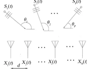
The approach taken here is to assume that the signal field at the array is comprised of P independent plane-wave arrivals from P known directions, as shown in Figure 1.

[image:1.595.350.492.604.717.2]

In practice, of course, the directions are rarely known

exactly, however this difficulty can be overcome by us- ing the standard MUSIC algorithm [5,6], which consti- tutes an angular pseudo-spectrum and an indicator of directions of arrival of different signals. The problem then reduces to estimating the signal powers from each of the P directions.

This study focuses on developing estimators which are used to identify the distribution of signal power gener- ated by acoustic sources. This paper is organized as fol- lows. An array signal model and the spatial covariance matrix of the sensor outputs are formulated in Section 2. The conventional beamformer and adaptive beamformers are presented respectively in Sections 3 and 4. A tech- nique to obtain the strengths of signals arriving at an ar- ray of sensors based on the covariance vector of signals is developed in Section 5. A signal power estimation obtained by the pseudoinverse of the array manifold ma- trix is studied in Section 6. Numerical and experimental results showing the effectiveness and the weakness of different algorithms in signal power estimation are pre- sented in Section 7. This paper is briefly concluded in Section 8.

2. Signal Representation and Sensor Output

Covariance Matrix

Consider a uniform linear array with N sensors (Figure 1). Assume that P acoustical plane waves at frequency f impinge upon the array from P different directions





θ1, , θp . The complex envelope of the kth sensor’s output is [3-5]

 

 





 

1

2π

exp 1 sin ,

1, 2, ,

P

k i i k

i

x t s t j d k n t

k N

 



 

 _  _

 









(1)

where the meanings of the various parameters are as fol- lows: s ti

 

is the complex envelope of the ith signal

source at the first sensor; d is the space between two ad- jacent sensors; is the signal wavelength correspond- ing to frequency f and n t is the additive noise output of the kth sensor.

λ

 

k

The complex envelope of the ith source is a zero-mean complex random variable. Its variance, denoted pi, char- acterizes the signal power of the ith source which we wish to estimate

 

   

Var

i i i i

p  _s t _E s t s t_ _ (2)

Here, E

 

is the expectation operator and the su- perscript * _{represents the complex conjugate.}

Equation (1) can also be expressed in the vector form as the N-dimensional vector [3]

 

 

   

1 P

i i

i

t s t 







x a n t (3)

where

 

 

 

T

 

 

 

T

1 , , N , 1 , , N

t _x t x t _ t _n t n t 

x  n  _

Here, T denotes transpose, and the direction of arrival of the ith signal source is represented by the N-dimen- sional complex vector a

 

_i . The noise is assumed to be spatially white (uncorrelated from sensor to sensor) and the same power level is present in each receiver. With these assumptions, the covariance matrix for the noise alone is given by Rn En

   

t n t H pnI ,



where n is the noise power, the identity matrix and the superscript H denotes the Hermitian transpose operation. Equation (3) may be rewritten in the matrix form

p I



N N

 

t 

  

t 

x As n t



(4) A is the



N P



array manifold matrix containing the manifold vectors for different sources as its columns,

 

1 , ,

 

P

 _ _.For any single plane wave arri- val, the outputs from the N individual receivers will dif- fer in phase by an amount determined by the geometry of the array and the arrival direction. In other words, the elements Akr of the matrix Aare known functions of the signal arrival angles and the array elements locations. It can readily be seen that the output signal from the qth sensor may be written as

A a  a

 

 

 

1 P

q qr r

i q

x t A s t n







 t (5)

Since the P arrivals are by assumption independent, the source covariance matrix is given by

   

H





1

diag , ,

s E t t  p pP

R s s  (6)

and the diagonal elements are the powers of the sources , from the P directions, which we wish to estimate. The spatial covariance matrix of the receiver outputs can be expressed, for signals uncorrelated of each other and of noise, as

   

H H

s n

E t t 

 _{ } 

R x x AR A R (7)

In practice, the spatial covariance matrix is estimated by a finite number of time domain samples (snapshots) and the following estimated form is used

   

H 1

1

ˆ T

i i

i

t t

T 





R x x (8)

covariance matrix [3].

3. Conventional Beamformer

The conventional beamformer, also called the “time de- lay and sum” or “unweighted add-squared” beamformer, consists of a system of delay and sum networks which are designed to make the signals from the beamformer direction in phase at each sensor. The directional data

 

j

s t from direction j must be estimated from the sen- sors output data vector . The usual approach is to find a matrix , such that reconstructs the directional data, and for a conventional beamformer the equation is [8]

 

t

x

M s

 

t Mx

 

t

 

1 H

 

CB t N 

s A x t (9)

A power estimate for the signals can be found by forming the covariance matrix

   

H H 2

1

sCBE CB t CB t _N

R s s A RA (10)

and the strength of the ith source estimated by the con- ventional beamformer is

 

H

 

2

1

iCB i i

p

N  

 a Ra (11)

However, this leads to a biased estimate, as can be seen by substituting (7) into (10)



H H

2

1

sCB s n

N 

R A AR A R



A (12)

So unless and n , neither of which is generally the case, then the estimate will be biased.

H _N

A A I R 0

4. Minimum Variance Beamformer

The conventional beamformer can be considered as a kind of linear spatial filter with data- independent coeffi- cients. In contrast, the minimum variance beamformer, called also the standard Capon beamformer [3], can be considered has a kind of data-dependent spatial filter, in which the coefficients, represented by the weight vector

w of the array element outputs, are chosen such that the filter has a constant gain at a particular direction i while its output power is minimized. The constraint en- sures that the signal power coming from the ith source will be reproduced in undistorted form in the processor output. Thus, the beamformer tries to eliminate as best it can all the signals received at the sensors except the sig- nal coming from the ith wanted source. The weight vec- tor w is selected so as to minimize the output power of the array

H H H

minE_  _

w w xx w w Rw (13)

subject to the constraint

 

H ₁

i

 

w a (14)

By the method of Lagrange’s multiplier, it can be shown that the optimum weight vector is

   



H

 



1

1 1

i i i

   

 



w R a a R a (15)

and the power of the ith source estimated by the standard Capon beamformer is

 

H 1

 

1 iSCB

i i

p

  



a R a (16)

The standard Capon beamformer has better resolution than the conventional beamformer provided that the array steering vector corresponding to the signal of interest is accurately known. However, the performance of this tra- ditional adaptive beamformer can degrade seriously in practice when errors exist in the signal of interest steer- ing vector, which may be due to look direction error, array sensor position error and small mismatches in the sensor responses. In such cases the signal of interest might be mistaken as an interference signal and might be suppressed. A robust Capon beamforming algorithm [9], which is a natural extension of the standard Capon algo- rithm, is presented to overcome this difficulty. In the robust Capon beamforming algorithm we suppose that

 

i

a is the true direction vector of the ith source,

 

i

a is the assumed direction of the ith source and we consider that a

 

i is in the vicinity of a

 

i . This

can be expressed mathematically by the following ine- quality: a

   

i a i 2, where  is a bound con- trolling the uncertainty in the assumed look direction. To derive the robust Capon beamforming algorithm we use the reformulation of the standard Capon beamforming problem to which we append the previous inequality. We have the following minimization problem

H min

w w Rw (17)

subject to the constraint

   

2

i i

   

a a (18)

The optimization problem can be rewritten as the fol- lowing form

 

H 1

 

min i i



a a R a (19)

subject to the constraint (18). We consider the solution on the boundary of the constraint set and we reformulate the optimization problem as the following quadratic form with a quadratic equality constraint

 

H ₁

 

min_a a i R a i subject to

   

2

i i

   

a a

grange’s multiplier which is based on the cost function

 

 

H 1

 



   

2



i i i i

f _{a a}  _{R a}  _ _a  _a 

_

 ₍₂₁₎

Differentiating (21) with respect to a

 

i and equat-

ing to zero gives the optimal solution

 

 





1 _H

 

i i i

   

  

a a U I  U a  (22)

where and are matrice

nvectors a

U

e



n





N N

lues o

s containing the eig d eigenva f the covariance ma- trix R and  is the Lagrange multiplier. Using (22) in th quality constraint of (20) the Lagrange multiplier is obtained as the solution to the constraint equation





e e

 

2 1 H

i

   

 

U I Γ U a (23) The signal power estimation of the ith so

ro

urce using the bust Capon beamformer is then

 

H



_{2 1 2}



1 _H

 

1 2 iRCB i p λ i        

a U I   U a (24)

In summary of this section, the standard Capon beam- fo

5. Signal Power Estimation by the

Sin ers, the covari-

rmer is an optimal spatial filter that maximizes the signal to noise ratio, provided that the true covariance matrix and the array steering vector are accurately known. However, the covariance matrix can be inaccurately es- timated due to imperfect array calibrations, gain and phase errors in the sensors. The robust Capon beam- former presented in the paper can then be used in such situations for both signal power estimation and source location as shown in examples given in Section 7. An- other power estimator using the covariance vector of signals is presented in the next section.

Covariance Vector Estimator

ce we are interested in the signal pow

ance matrix of the data contains all the information about these signal strengths. The correlation between sensor k and l is rkl  E x x k l and from Equation (5) we obtrain

 

 

 

 

1 1

P P

k kj j k li i l

i i

r E A s t n t A s t n t

      _  _      





    

 (25)

But since signals from different directions must be un

N (26)

The sensor noise power on each sensor is constant and eq

correlated, we have

P 

1

; 1, , , 1, ,

kl i ki li n kl

i

r p A A p k N l







    

uals pn and  kl 1 for k l and zero otherwise. Equation (26) ma plit in l and imaginary com-

 





Re P Re p

y be s to rea

1

kl ki li i n kl

i

r A A p  (27)









 





1

Im kl P Im ki li i

i

r A A







2

p

Of the 2N equations represented by

(28)

(27) and (28) only



_N2_{ N 1}



ge

equations are independent. Indeed, one ts

 

Re

 

rlk ,k1, , ; N l1, , N (29) Re rkl

 

 

Im rkl  Im rlk ,k1, , ; N l1, , N (30)

 

 

Im rkk 0,k1, , Nand Re rkk Re

 

rll ,k l (31) Equations (27) and (28) may then be written form

in the



r Bp (32) where r, B and pare reals. r is

which contains the real and i

the



N  N 1



vector maginary components of

2

 

rkl and is called the covariance vector; p is the



P1



vector containing the signal powers

 

pi and

r noise power pn. Note that if the sensor noise is t may be desirable to omit the model of sensor noise. B is the

senso small, i



_N2_{  N 1}





_P1



_{matrix which con-}

tains all the array geometry terms and kl if required





Re A Aki li kl





Im A Aki li 0

           

B (33)

The least squares solution to (32) is

(34)

pCV is the vector containing the str the covariance vector. Performances

ation by the

Pseudo-Inverse of the Array Manifold

Fro

given by



T



T

CV

p B B 1B r

engths of signals by of this estimator are given in Section 7. Another power estimator based on the pseudoinverse of the array manifold matrix A is pre- sented in the next section.

6. Signal Power Estim

Matrix

m Equation (7) we obtain

H

s   n p

AR A R R R nI (35)

A possible approach to estimate the

to select the P diagonal elements of t s ge

signal strengths is he matrix R. We t

















1 1

H H H

H s n n        

A A A R R A A A A R R A

R

(36)

where A+ _{is the pseudoinverse of the array manifold ma-} trix. To obtain the noise covariance matrix RnpnI, or value decom- the noise power pn, we consider the eigen

position of the covariance matrix R

 



H



s pn

 R  AR A  I (37)

The rank of H s

AR A is equal to the number of inci- dent signals P and can be determined from the P largest eigenvalues of R. The minimum eigenvalue of R corre- sponds to the noise power pn.

Numerical simulations and experime

pr h

mental Results

stimator (CV) and the pseudoin- e rs. In ntal tests are now esented to evaluate t e performances of the estimators presented in the paper.

7. Numerical and Experi

The conventional beamformer (CB), the standard Capon beamformer (SCB), the robust Capon beamformer (RCB), the covariance vector e

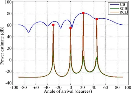
verse estimator (PI) are employed to estimate th strengths of signals arriving at an array of receive our simulations, we assume a uniform linear array with N = 6 omnidirectional sensors and half-wavelength sensor spacing. Four point sources are located at bearings of— 30˚, 0˚, 22˚ and 45˚. The source powers are respectively 60 dB, 55 dB, 80 dB and 70 dB and the number of snap- shots is T = 4096. The signal to noise ratio is SNR = 20

dB. Figure 2 shows the power estimates of CB, SCB and

[image:5.595.310.536.327.488.2]

RCB as a function of the direction angle in the case where there are no gain and phase errors in the sensors of the array. The small circles denote the true direction of arrival and the true power of the four sources. The SCB and RCB estimators provide excellent power estimates of the incident sources and can also be used to determine their directions of arrival based on the peak power loca-

Figure 2. Power estimates versus the steering direction θ using CB, SCB and RCB without gain and phase errors and SNR = 20 dB.

tions. The CB estimator has much poorer resolution than both SCB and RCB and the sidelobes of the former give false peaks and false directions of arrival of sources.

Figure 3 shows the power estimates of CB, SCB and

RCB in the case where there are a gain error of 0.02 and a phase error 0.2˚ in each sensor. We note that SCB and RCB can still give good direction of arrival estimates for the incident signals based on the peak locations, however, the SCB estimates of the incident signal powers are way off. In this case, only the RCB algorithm gives good power estimates of the incident sources and can also be used to determine their directions of arrival based on the peak locations.

The remaining part of the section is focused on the ap- plication of the developed algorithms to the experimental identification of noise sources generated by two loud

s (the loudspeakers) in the anechoic room. - speakers. The experimental setup is schematically shown in the block diagram of Figure 4 with the acoustic array and two source

Figure 3. Power estimates versus the steering direction θ using CB, SCB and RCB with 0.02 gain error and 0.2˚

[image:5.595.60.286.512.694.2]

phase error in each sensor and SNR = 20.

[image:5.595.311.535.539.719.2]

The receiving acoustic array is linear and formed with six omnidirectional microphones equally spaced, with

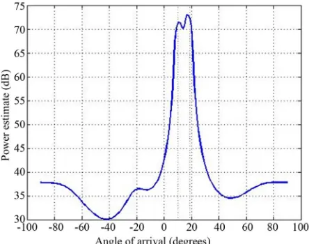
ter-element spacing of d = 4.5 cm. The two acoustic sources (the loudspeakers) and the acoustic array are in the same horizontal plane. The transmitting loudspeakers generate two typical audio signals at a frequency of 3800 Hz corresponding to a microphone separation distance of one-half wavelength. The number of snapshots is T = 4096. We are able to find the direction of the two sources by using the MUSIC algorithm, however, unlike the methods mentioned earlier, MUSIC does not physically correspond to the signal power. The MUSIC algorithm is only an indicator of directions of arrival of different sig- nals. Figure 5 shows the normalized angular spectrum function obtained from MUSIC where important peaks appear at the signal directions. We obtain the angular position of the sources and

Once the arrival angl been ed we ca es

in

1 10

  

es have 2

19

  _.

determin n

ti ur

proposed algorithms. Table 1 shows the results obtained by our algorithms.

[image:6.595.312.534.88.263.2] [image:6.595.60.285.451.628.2]

The experimental results confirm that the CV and the PI estimators give very similar results and the RCB esti- mator overestimates very slightly the source powers.

Figure 6 shows the power estimates versus the steer-

ing direction using the RCB algorithm. From this plot we obtain simultaneously an estimate of directions of arrival and an estimate (slightly overestimated) of the power of the two sources, based on the two peak locations.

mate the power of the two acoustic sources by o

[image:6.595.57.287.675.734.2]

Figure 5. Experimental MUSIC spatial spectra.

Table 1. Power estimation using different estimators.

Estimator RCB CV PI

Source 1, 110 72.1 dB 70.9 dB 70.8 dB



Source 2, 219 73 dB 71.8 dB 71.8 dB



F

8.

Five s essors to ate the strengths of signals

arri an array of have stud he

conve beamform he standard Capon beam-

fo ide in gene or po imat e

incident sources. The robust Capon beamformer gives good power estimates and can also be used to determine the directions of arrival of incident sources. The covari- ance vector and the pseudoinverse estimators give excel- lent power estimates. From numerical simulations and field tests, the RCB, CV and PI algorithms exhibit re- markable effectiveness in finding the strengths of signals. The performances of these algorithms in the case of very close sources are under investigation.

These techniques have been developed for the estima- tion of signal strengths using an array of receivers. How- ever, the principles can be applied to a wide range of other estimation problems, of which the spectrum analy- sis of a time series is an example.

REFERENCES

[1]

9.

igure 6. Experimental robust capon beamformer.

Conclusions

ignal proc estim ving at

ntional

sensors er and t

been ied. T

rmer prov ral po wer est es of th

F. J. Fay, “Sound Intensity,” Elsevier Applied Science, Amsterdam, 198

[2] M. R. Bay, “Application of BEM-Based Acoustic Holo- graphy to Radiation Analysis of Sound Sources with Ar- bitrarily Shaped Geometries,” Journal of the Acoustical Society of America,Vol. 92, No. 1, 1992, pp. 533-549.

doi:10.1121/1.404263

[3] P. Stoica and R. Moses, “Spectral Analysis of Signals,” Prentice Hall, Upper Saddle River, 2005.

[4] T. J. Shan, M. Wax and T. Kailath, “On Spatial Smooth- ing for Direction of Arrival Estimation of Coherent Sig- nals,” IEEE Transactions on Acoustic, Speech and Signal Processing, Vol. 33, No.4, 1985, pp. 806-811.

doi:10.1109/TASSP.1985.1164649

6, pp. 276-280. Parameter Estimation,” IEEE Transactions on Antennas and Propagation, Vol. 34, No. 3, 198

doi:10.1109/TAP.1986.1143830

[6] P. Stoica, Z. Wang and J. Li, “Extended Derivation of MUSIC in the Presence of Steering Vector Errors,” IEEE Transactions on Signal Processing, Vol. 53, No. 3, 2005, pp. 1209-1211. doi:10.1109/TSP.2004.842201

[7] M. Yang, M. Al-Kutubi and D. T. Pham, “In-Solid Acoustic Source Localization Using Likelihood Mapping

Algorithm,” Open Journal of Acoustics, Vol. 1, 2011, pp. 34-40. doi:10.4236/oja.2011.12005

[8] H. A. d’Assumpcao an G. E. Mountford, “An Overview

bust Capon Beamform- of Signal Processing for Arrays of Receivers,” Journal of Electrical and Electronics Engineering,Vol. 4, No. 1, 1984, pp. 6-18.

[9] J. Li, P. Stoica and Z. Wang, “Ro