Munich Personal RePEc Archive
Analogy Making, Option Prices, and
Implied Volatility
Siddiqi, Hammad
1 July 2013
1
Analogy Making, Option Prices, and Implied Volatility
Working Paper
This version: July 2013
Previous versions circulated as “Coarse Thinking, Implied Volatility, and the Price of Call and Put Options” and “Thinking by Analogy and Option Prices”
Hammad Siddiqi1
Lahore University of Management Sciences
hammad@lums.edu.pk
Abstract
We put forward a new option pricing formula based on the notion that people tend to think by analogies and comparisons. The new formula differs from the Black Scholes formula due to the appearance of a parameter in the formula that captures the risk premium on the underlying. The new formula, called the analogy option pricing formula, provides an explanation for the implied volatility skew puzzle in equity options. We also discuss the key empirical predictions of the analogy formula.
Keywords: Analogy Making, Implied Volatility, Implied Volatility Skew, Option Prices, Risk Premium
JEL Classifications: G13; G12
1
2
Analogy Making, Option Prices, and Implied Volatility
People tend to think by analogies and comparisons. It has been argued in cognitive science and
psychology literature that analogy making forms the core of human cognition and it is the fuel and
fire of thinking (see Hofstadter and Sander (2013)). Hofstadter and Sander (2013) write, “[…] each concept in our mind owes its existence to a long succession of analogies made unconsciously over many years, initially giving birth to the concept and continuing to enrich it over the course of our lifetime. Furthermore, at every moment of our lives, our concepts are selectively triggered by analogies that our brain makes without letup, in an effort tomake sense of the new and unknown in terms of the old and known.”
(Hofstadter and Sander (2013), Prologue page1).
According to Hoftsadter and Sander (2013), we engage in analogy making when we spot a
link between what we are just experiencing and what we have experienced before. For example, if
we see a pencil, we are able to recognize it as such because we have seen similar objects before and
such objects are called pencils. Furthermore, spotting of this link is not only useful in assigning
correct labels, it also gives us access to a whole repertoire of stored information regarding pencils
including how they are used and how much a typical pencil costs. Hofstadter and Sander (2013)
argue that analogy making not only allows us to carry out mundane tasks such as using a pencil,
toothbrush or an elevator in a hotel but is also the spark behind all of the major discoveries in
mathematics and the sciences. They argue that analogy making is responsible for all our thinking,
from the most trivial to the most profound. Of course, there is always a danger of making wrong
analogies. When a small private plane flew into a building in New York on October 11, 2006, the
analogy with the events of September 11, 2001 was irrepressible and the Dow Jones Index fell
sharply in response.
Recent experimental evidence suggests that analogy making plays an important role in
financial markets. Siddiqi (2012) and Siddiqi (2011) show through controlled laboratory experiments
that analogy making strongly influences how much people are willing to pay for call options. These
experiments exploit an analogy between in-the-money call options and their underlying stocks and
show that in-the-money calls are overpriced due to participants forming an analogy between riskier
options and comparatively less risky underlying stocks.
In this article, we investigate the theoretical implications of analogy making for option
3 pricing formula (alternative to the Black Scholes formula) is obtained. The new formula, which we
call the analogy option pricing formula, provides an explanation for the implied volatility skew
puzzle. Interestingly, the new formula differs only slightly from the Black-Scholes formula by
incorporating the risk premium on the underlying in option price. This additional parameter is
sufficient to explain implied volatility. We also provide testable predictions of the analogy option
pricing formula.
This paper adds to the literature in several ways. 1) We show how a particular bias, called
analogy making, leads to a new option pricing formula and explains the implied volatility puzzle. In
particular, we show that the implied volatility skew is generated if actual price dynamics are
determined according to the analogy formula and the Black-Scholes formula is used to back-out
implied volatility. Our approach is broadly consistent with Shefrin (2008) who provides a systematic
treatment of how behavioral assumptions impact the pricing kernel at the heart of modern asset
pricing theory. However, the treatment here differs from Shefrin (2008) as we focus on one
particular bias and explore its implications. 2) We provide a number of testable predictions of the
model and summarize existing evidence. The existing evidence is strongly favorable to the analogy
approach. Robust empirical testing of these predictions is the subject of future research. 3) Our
approach relates to Bollen and Whaley (2004). They argue that, in the presence of limits to arbitrage,
net demand pressure could determine the level and the slope of the implied volatility curve. In our
approach, the source of demand pressure behind the skew is analogies that investors make between
in-the-money calls and the underlying stocks. Such analogies lead them to consider in-the-money
calls as replacements of the underlying stocks.2 4) Duan and Wei (2009) use daily option quotes on
the S&P 100 index and its 30 largest component stocks, to show that, after controlling for the underlying asset’s total risk, a higher amount of systematic risk leads to a higher level of implied volatility and a steeper slope of the implied volatility curve. In the analogy option pricing model,
higher risk premium for a given level of historical volatility generates this result. As risk premium is
related to systematic risk, this prediction of the analogy model is quite intriguing. 5) Our approach is
an example of behavioralization of finance. Shefrin (2010) argues that finance is in the midst of a
2
Option traders and investment professionals often advise people to buy in-the-money calls rather than the underlying stocks. As illustrative examples, see the following:
http://ezinearticles.com/?Call-Options-As-an-Alternative-to-Buying-the-Underlying-Security&id=4274772,
http://www.investingblog.org/archives/194/deep-in-the-money-options/,
http://www.triplescreenmethod.com/TradersCorner/TC052705.asp,
4 paradigm shift, from a neoclassical based framework to a psychologically based framework.
Behavioralizing finance is the process of replacing neoclassical assumptions with behavioral
counterparts.
In general, pricing models that have been proposed to explain the implied volatility skew can
be classified into three broad categories: 1) Stochastic volatility and GARCH models (Heston and
Nandi (2000), Duan (1995), Heston (1993), Melino and Turnbull (1990), Wiggins (1987), and Hull
and White (1987)). 2) Models with jumps in the underlying price process (Amin (1993), Ball and
Torous (1985)). 3) Models with stochastic volatility as well as random jumps. See Bakshi, Cao, and
Chen (1997) for a discussion of their empirical performance (mixed). Most of these models modify
the price process of the underlying. Hence, the focus of these models is on finding the right
distributional assumptions that could explain the implied volatility puzzles. Our approach differs
from them fundamentally as we do not modify the underlying price process. That is, as in the Black Scholes model, we continue to assume that the underlying’s stochastic process is a constant
coefficient geometric Brownian motion. To our knowledge, ours is the only model that explains the
implied volatility skew without modifying the geometric Brownian motion assumption of the
Black-Scholes model. Hence, contrary to popular belief, explaining implied volatility does not require that
the assumption of geometric Brownian motion for the underlying is modified.
Analogy making is likely to play an important role in understanding financial market
behavior. Many researchers have pointed out that there appears to be clear departures from Bayesian
thinking (Babcock & Loewenstein (1997), Babcock, Wang, & Loewenstein (1996), Hogarth &
Einhorn (1992), Kahneman & Frederick (2002), Kahneman, Slovic, & Tversky (1982)). Such
departures from rational thinking have been measured both at the individual as well as the market
level (Siddiqi (2009), Kluger & Wyatt (2004)). However, the question of what type of behavior to
allow for if non-Bayesian behavior is admitted is a difficult one to address in the absence of an
alternative which is amenable to systematic analysis. Analogy making may provide such an
alternative especially when its intuitive appeal is undeniable.
This paper is organized as follows. Section 1 illustrates the difference between the principle
of no arbitrage and the principle of analogy making through a simple example. Section 2 develops
the key ideas in this paper in the context of a one period binomial model. Section 3 puts forward the
analogy option pricing formula. Section 4 shows if prices are determined in accordance with the
5 volatility skew is observed. Section 5 puts forward the key empirical predictions of the model.
Section 6 concludes.
1. An Example: Principle of No-Arbitrage vs. Principle of Analogy Making
Consider an investor who has initially put his money in two assets: A stock (S) and a risk free bond
(B). The stock has a price of $140 today. In the next period, the stock could either go up to $200
(the red state) or go down to $90 (the blue state). Each state has a 50% chance of occurring. The
bond costs $100 today and it also pays $100 in the next period implying a continuously compounded
interest rate of zero. Suppose a new asset “A” is introduced to him. The asset “A” pays $140 in the
red state and $30 in the blue state. How much should he be willing to pay for it?
Conventional finance theory provides an answer by appealing to the principle of
no-arbitrage: identical assets should offer the same returns. An asset identical to “A” is a portfolio consisting of a long position in S and a short position in 0.60 of B. In the red state, S pays $200 and one has to
pay $60 due to shorting 0.60 of B resulting in a net payoff of $140. In the blue state, S pays $90 and
one has to pay $60 on account of shorting 0.60 of B resulting in a net payoff of $30. That is, payoffs
from S-0.60B are identical to payoffs from “A”. Hence, according to the no-arbitrage principle, “A”
should be priced in such a way that its expected return is equal to the expected return from
(S-0.60B). It follows that the no-arbitrage price for “A” is $80.
In practice, finding an asset identical to A is no easy task. When simple tasks such as the one
described above are presented to participants in a series of experiments, they seem to rely on
analogy-making to figure out their willingness to pay. See Siddiqi (2012) and Siddiqi (2011). So,
instead of trying to construct a hypothetical asset which is identical to asset “A”, people find an
actual asset similar to “A” and price “A” in analogy with that asset. That is, they rely on the principle
of analogy: similar assets should offer the same returns rather than on the principle of no-arbitrage: identical assets should offer the same returns.
Asset “A” is similar to asset S. It pays more when asset S pays more and it pays less when
asset S pays less. Expected return from S is 1.0357
. According to the principle of
analogy, A’s price should be such that it offers the same expected return as S. That is, the right price
6 In the above example, there is a gap of $2.07 between the no-arbitrage price and the analogy
price. Rational investors should short “A” and buy “S-0.60B”. However, if we introduce a small
transaction cost of 1%, then the total transaction cost of the proposed scheme exceeds $2.07, preventing arbitrage. The transaction cost of shorting “A” is $0.8207 whereas the transaction cost of buying “S-0.60B” is $1.6 so the total transaction cost is $2.4207. Hence, in principle, the deviation between the no-arbitrage price and the analogy price may not be corrected due to transaction costs.
Next, we illustrate the key ideas in a binomial context.
2. Analogy Making: The Binomial Case
Consider a simple two state world. The equally likely states are Red, and Blue. There is a stock with
payoffs corresponding to states Red, and Blue respectively. The state realization takes
place at time . The current time is time . We denote the risk free discount rate by . The current
price of the stock is . There is another asset, which is a call option on the stock. By definition, the
payoffs from the call option in the two states are:
Where is the striking price, and are the payoffs from the call option corresponding to
Red, and Blue states respectively.
As can be seen, the payoffs in the two states depend on the payoffs from the stock in
corresponding states. Furthermore, by appropriately changing the striking price, the call option can
be made more or less similar to the underlying stock with the similarity becoming exact as
approaches zero (all payoffs are constrained to be non-negative). As our focus is on in-the-money
call options, we assume:
How much is an analogy maker willing to pay for this call option?
An analogy maker co-categorizes this call option with the underlying and values it in transference with the underlying stock. In other words, an analogy maker relies on the principle of analogy: similar assets should offer the same return. In contrast, a rational investor relies on the principle of no-arbitrage:
7 We denote the return on an asset byqQ, whereQis some subset of (the set of real
numbers). In calculating the return of the call option, an analogy maker faces two similar, but not
identical, observable situations, s{0,1}. Ins0, “return demanded on the call option” is the
attribute of interest and ins 1, “actual return available on the underlying stock” is the attribute of
interest. The analogy maker has access to all the information described above. We denote this public
information by .
The actual expected return available on the underlying stock is given by,
For the analogy maker, the expected return demanded on the call option is:
So, the analogy maker infers the price of the call option, , from:
It follows,
We know,
where δ is the risk premium on the underlying.
8
The above equation is the one period analogy option pricing formula for in-the-money binomial
case.
The rational price is (from the principle of no-arbitrage):
If limits to arbitrage prevent rational arbitrageurs from making riskless profits at the expense of
analogy makers, both types will survive in the market. If is the weight of rational investors in the
market price and is the weight of analogy makers, then the market price becomes:3
Proposition 1 The price of a call option in the presence of analogy makers ( ) is always
larger than the price in the absence of analogy makers ( ) as long as the underlying
stock price reflects a positive risk premium. Specifically, the difference between the two
prices is where δ is the risk premium reflected in the
price of the underlying stock.
Proof.
Subtracting equation (8) from equation (9) yields the desired expression which is greater than zero as
long as .
▄
Proposition 2 shows that the presence of analogy makers does not change the Sharpe-ratio of
options. This shows that the mispricing of options with respect to the underlying due to the
presence of analogy makers is not reflected in the Sharpe-ratio as the change in expected excess
return is offset by the change in standard deviation.
3
9 Proposition 2 The Sharpe-ratio of a call option remains unchanged regardless of whether the
analogy makers are present or not. Specifically, the Sharpe-ratio remains equal to the
Sharpe-ratio of the underlying regardless of the presence of analogy makers.
Proof.
Initially, assume that analogy makers are not present. Let be the number of units of the underlying
stock needed and let be the dollar amount invested in a risk-free bond to create a portfolio that
replicates the call option. It follows,
Substitute B from (I) into (II) and re-arrange to get:
Where is the elasticity of option’s price with respect to the stock price, and are returns on call and stock respectively. It follows,
10
=
If analogy makers are also present, it follows,
harpe ratio of all with analo y a ers r r r
▄
Proposition 2 shows that the mispricing caused by the presence of analogy makers does not change
the Sharpe-ratio. It remains equal to the Sharpe-ratio of the underlying. Hence, the fact that the
empirical Sharpe-ratios of call options and underlying stocks do not differ cannot be used to argue
that there is no mispricing in options with respect to the underlying.
Proposition 3 shows the condition under which rational arbitrageurs cannot make arbitrage profits
at the expense of analogy makers. Consequently, both types may co-exist in the market.
Proposition 3 Analogy makers cannot be arbitraged out of the market if
where c is the transaction cost involved in the
11 Proof.
The presence of coarse thinkers increases the price of an in-the-money call option beyond its
rational price. A rational arbitrageur interested in profiting from this situation should do the
following: Write a call option and create a replicating portfolio. If there are no transaction costs
involved then he would pocket the difference between the rational price and the market price
without creating any liability for him when the option expires. As proposition 1 shows, the
difference is e e . However, if there are transactions costs involved
then he would follow the strategy only if the benefit is greater than the cost. Otherwise, arbitrage
profits cannot be made.
▄
Analogy makers overprice a call option. When such overpriced calls are added to portfolios then the
dynamics of such portfolios would be different from the dynamics without overpricing. Proposition
4 considers the case of covered call writing and shows that the two portfolios grow with different
rates with time.
Proposition 4 If analogy makers set the price of an in-the-money call option then the
covered call writing position (long stock+short call) grows in value at the rate of . If
rational investors set the price of an in-the-money call option then the covered call writing
position grows in value at the risk free rate .
Proof.
Re-arranging equation (8):
The right hand side of the above equation is the covered call writing position with rational pricing.
Hence, it follows that the covered call portfolio grows in value at the risk free rate with time if
investors are rational.
12
The right hand side of the above equation is the covered call writing position when analogy makers
price the call option. As the left hand side shows, this portfolio grows at a rate of with time.
▄
Proposition 4 is useful in developing intuition regarding the derivation of the option pricing formula
when we consider the general case, which we turn to next.
3. The Option Pricing Formula
In this section, we derive a new option pricing formula by allowing the underlying to follow a
geometric Brownian motion instead of the restrictive binomial process assumed in the previous
section. By exploring the implications of analogy making in the binomial case, the previous section
develops intuition which carries over to the general case discussed here. Two results from the
previous section stand out in this respect. Firstly, the rational and the analogy price differ in one parameter only, δ, which is the risk premium on the underlying stock. The analogy price is larger than the rational price if risk premium is positive (proposition 1). Secondly, for in-the-money call
options, the covered call portfolio grows at the rate in the analogy case, rather than the rate ,
which holds in the rational case (proposition 4).
To simplify notation, in this section, we are denoting the price of a call option by and the
price of a put option by with the context making clear whether we are talking about the analogy
price or the rational price. All other notations carry over from the previous section. Furthermore, we
are only discussing European options.
In the binomial world, the portfolio grows at the risk free rate with time under
rational pricing whereas it grows at the rate with time under analogy pricing ( is the delta of
call option, which is equal to 1 for an in-the-money binomial situation). Proposition 5 considers the
corresponding case when the underlying follows geometric Brownian motion and derives the
13 Proposition 5 The Analogy Option Pricing Partial Differential Equation (PDE) is
Proof.
See Appendix A
▄
The analogy option pricing PDE can be solved by transforming it into the heat equation.
Proposition 6 shows the resulting call option pricing formula for European options.
Proposition 6 The formula for the price of a European call is obtained by solving the
analogy based PDE. The formula is where
and
Proof.
See Appendix B.
▄
Corollary 6.1 The formula for the analogy based price of a European put option is
The analogy option pricing formula is different from the Black-Scholes formula due to the
appearance of risk premium on the underlying in the analogy formula. It suggests that the risk
premium on the underlying stock does matter for option pricing. The analogy formula is derived by
keeping all the assumptions behind the Black-Scholes formula except one: the no-arbitrage pricing.
That is, the analogy price deviates from the no-arbitrage price, however, as the next section
illustrates, the deviation may not be large enough to justify an arbitrage scheme in the presence of
14 4. The Implied Volatility Skew
All the parameters and variables in the Black Scholes formula are directly observable except for the standard deviation of the underlying’s returns. So, by plugging in the values of observables, the value of standard deviation can be inferred from market prices. This is called implied volatility. If the
Black Scholes formula is correct, then the implied volatility values from options that are equivalent
except for the strike prices should be equal. However, in practice, a skew is observed in which
in-the-money call options’ (out-of-the money puts) implied volatilities are higher than the implied
volatilities from at-the-money and out-of-the-money call options (in-the-money puts).
The behavioral approach developed here provides an explanation for the skew. If the
analogy formula is correct, and the Black Scholes model is used to infer implied volatility then skew
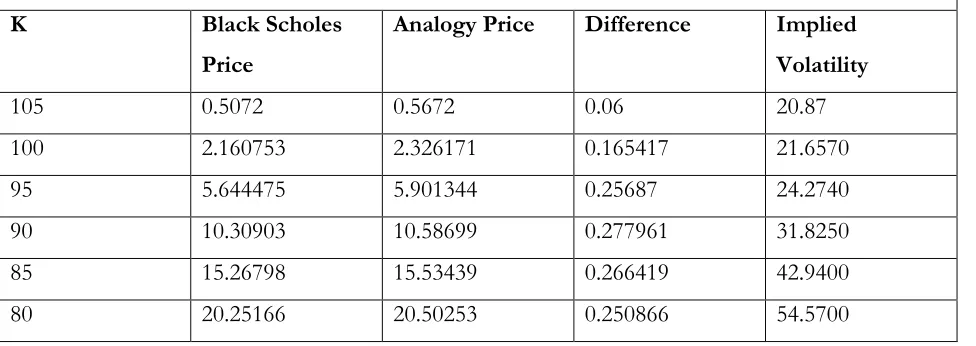
[image:15.612.67.555.398.571.2]arises as table 1 shows.
Table 1
Implied Volatility Skew
Underlying’s Price=100, Historical Volatility=20%, Risk Premium on the Underlying=5%, Time to Expiry=0.06 year
K Black Scholes
Price
Analogy Price Difference Implied
Volatility
105 0.5072 0.5672 0.06 20.87
100 2.160753 2.326171 0.165417 21.6570
95 5.644475 5.901344 0.25687 24.2740
90 10.30903 10.58699 0.277961 31.8250
85 15.26798 15.53439 0.266419 42.9400
80 20.25166 20.50253 0.250866 54.5700
As table 1 shows, implied volatility skew is seen if the analogy formula is correct, and the Black
Scholes formula is used to infer implied volatility. Notice that in the example considered, difference
between the Black Scholes price and the analogy price is quite small suggesting that transaction costs
15 K/S
Figure 1
Figure 1 is the graphical illustration of table 1. It is striking to observe from table 1 and figure 1 that
the implied volatility skew is quite steep even when the price difference between the Black Scholes
price and the analogy price is small. In the next section, we outline a number of key empirical
predictions that follow from the analogy making model.
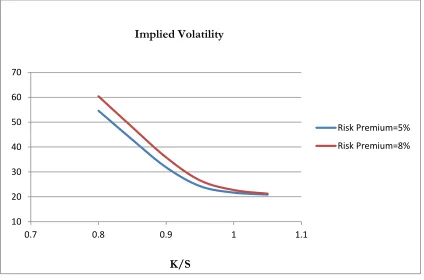
5. Key Predictions of the Analogy Model
Prediction#1 After controlling for the underlying asset’s total volatility, a higher amount of
risk premium on the underlying leads to a higher level of implied volatility and a steeper
slope of the implied volatility curve.
Risk premium on the underlying plays a key role in analogy option pricing formula. Higher the level
of risk premium for a given level of volatility; higher is the extent of overpricing. So, higher risk
premium leads to higher implied volatility levels at all values of moneyness. Figure 2 illustrates this.
In the figure, implied volatility skews for two different values of risk premia are plotted. Other
parameters are the same as in table 1. Duan and Wei (2009) use daily option quotes on the S&P 100
0 10 20 30 40 50 60
0.7 0.75 0.8 0.85 0.9 0.95 1 1.05 1.1
16 index and its 30 largest component stocks, to show that, after controlling for the underlying asset’s
total risk, a higher amount of systematic risk leads to a higher level of implied volatility and a steeper
slope of the implied volatility curve. As risk premium is related to systematic risk, the prediction of
[image:17.612.73.497.163.443.2]the analogy model is quite intriguing.
Figure 2
Prediction#2 Implied volatility should typically be higher than realized/historical volatility
It follows directly from the analogy formula that as long as the risk premium on the underlying is
positive, implied volatility should be higher than actual volatility. Anecdotal evidence is strongly in
favor of this prediction. Rennison and Pederson (2012) calculate implied volatilities from
at-the-money options in 14 different options markets over a period ranging from 1994 to 2012. They show
that implied volatilities are typically higher than realized volatilities.
Prediction#3 Implied volatility curve should flatten out with expiry
Figure 3 plots implied volatility curves for two different expiries. All other parameters are the same
as in table 1. It is clear from the figure that as expiry increases, the implied volatility curve flattens
out.
10 20 30 40 50 60 70
0.7 0.8 0.9 1 1.1
Risk Premium=5% Risk Premium=8%
Implied Volatility
17 Figure 3
Empirically, implied volatility curve typically flattens out with expiry (see Greiner (2013) as one
example). Hence, this match between a key prediction of the analogy model and empirical evidence
is quite intriguing.
6. Conclusion
Analogy making appears to be the key to the way we think. In this article, we investigate the
implications of analogy making for option pricing. We put forward a new option pricing formula
that we call the analogy option pricing formula. The new formula differs with the Black Scholes
formula due to the introduction of a new parameter capturing risk premium on the underlying stock.
The new formula provides an explanation for the implied volatility skew puzzle. Three testable
predictions of the model are also discussed. Rigorous testing of these predictions is the subject of
future research.
10 15 20 25 30 35 40 45 50 55 60
0.7 0.8 0.9 1 1.1
Expiry=0.06 Year Expiry=1 Year
Implied Volatility
18 References
Amin, K., 1993. Jump diffusion option valuation in discrete time. Journal of Finance 48, 1833-1863.
Babcock, L., & Loewenstein, G. (1997). “Explaining bargaining impasse: The role of self-serving biases”. Journal of Economic Perspectives, 11(1), 109–126.
Babcock, L., Wang, X., & Loewenstein, G. (1996). “Choosing the wrong pond: Social comparisons in
negotiations that reflect a self-serving bias”. The Quarterly Journal of Economics, 111(1), 1–19.
Bakshi G., Cao, C., Chen, Z., 1997. Empirical performance of alternative option pricing models. Journal of Finance 52, 2003-2049.
Ball, C., Torous, W., 1985. On jumps in common stock prices and their impact on call option pricing. Journal of Finance 40, 155-173.
Black, F., Scholes, M. (1973). “The pricing of options and corporate liabilities”. Journal of Political Economy 81(3): pp. 637-65
Black, F., (1976), “Studies of stock price volatility changes. Proceedings of the 1976 Meetings of the American Statistical Association, Business and Economic Statistics Section, 177–181.
Bollen, N., and R. Whaley. 2004. Does Net Buying Pressure Affect the Shape of Implied Volatility Functions?Journal of Finance 59(2): 711–53
Bossaerts, P., Plott, C. (2004), “Basic Principles of Asset Pricing Theory: Evidence from Large Scale Experimental Financial Markets”. Review of Finance, 8, pp. 135-169.
Carpenter, G., Rashi G., & Nakamoto, K. (1994), “Meaningful Brands from Meaningless Differentiation: The
Dependence on Irrelevant Attributes,” Journal of Marketing Research 31, pp. 339-350
Christensen B. J., and Prabhala, N. R. (1998), “The Relation between Realized and Implied Volatility”, Journal of Financial Economics Vol.50, pp. 125-150.
Christie A. A. (1982), “The stochastic behavior of common stock variances: value, leverage and interest rate effects”, Journal of Financial Economics 10, 4 (1982), pp. 407–432
DeBondt, W. and Thaler, R. (1985). “Does the Stock-Market Overreact?”Journal of Finance 40: 793-805
Derman, E. (2003), “The Problem of the Volatility Smile”, talk at the Euronext Options Conference available
at http://www.ederman.com/new/docs/euronext-volatility_smile.pdf
Derman, E., Kani, I., & Zou, J. (1996), “The local volatility surface: unlocking the information in index option prices”, Financial Analysts Journal, 52, 4, 25-36
Duan, Jin-Chuan, and Wei Jason (2009), “Systematic Risk and the Price Structure of Individual Equity
Options”, The Review of Financial studies, Vol. 22, No.5, pp. 1981-2006.
Duan, J.-C., 1995. The GARCH option pricing model. Mathematical Finance 5, 13-32.
Dumas, B., Fleming, J., Whaley, R., 1998. Implied volatility functions: empirical tests. Journal of Finance 53, 2059-2106.
19 Fama, E.F., and French, K.R. (1988). “Permanent and Temporary Components of Stock Prices”. Journal of Political Economy 96: 247-273
Fleming J., Ostdiek B. and Whaley R. E. (1995), “Predicting stock marketvolatility: a new measure”. Journal of Futures Markets 15 (1995), pp. 265–302.
Greiner, S. P. (2013), “Investment risk and uncertainty: Advanced risk awareness techniques for the intelligent investor”. Published by Wiley Finance.
Han, B. (2008), “Investor Sentiment and Option Prices”, The Review of Financial Studies, 21(1), pp. 387-414.
Heston S., Nandi, S., 2000. A closed-form GARCH option valuation model. Review of Financial Studies 13, 585-625.
Heston S., 1993. “A closed form solution for options with stochastic volatility with application to bond and
currency options. Review of Financial Studies 6, 327-343.
Hofstadter, D., and Sander, E. (2013), “Surfaces and Essences: Analogy as the fuel and fire of thinking”,
Published by Basic Books, April.
Hogarth, R. M., & Einhorn, H. J. (1992). “Order effects in belief updating: The belief-adjustment model”. Cognitive Psychology, 24.
Hull, J., White, A., 1987. The pricing of options on assets with stochastic volatilities. Journal of Finance 42, 281-300.
Kahneman, D., & Frederick, S. (2002). “Representativeness revisited: Attribute substitution in intuitive
judgment”. In T. Gilovich, D. Griffin, & D. Kahneman (Eds.), Heuristics and biases (pp. 49–81). New York: Cambridge University Press.
Kahneman, D., & Tversky, A. (1982), Judgment under Uncertainty: Heuristics and Biases, New York, NY: Cambridge University Press.
Kluger, B., & Wyatt, S. (2004). “Are judgment errors reflected in market prices and allocations? Experimental evidence based on the Monty Hall problem”. Journal of Finance, pp. 969–997.
Lakoff, G. (1987), Women, Fire, and Dangerous Things, Chicago, IL: The University of Chicago Press.
Lettau, M., and S. Ludvigson (2010): Measuring and Modelling Variation in the Risk-Return Trade-off" in Handbook of Financial Econometrics, ed. by Y. Ait-Sahalia, and L. P. Hansen, chap. 11,pp. 617-690. Elsevier Science B.V., Amsterdam, North Holland.
Lustig, H., and A. Verdelhan (2010), “Business Cycle Variation in the Risk-Return
Trade-off". Working paper, UCLA.
Melino A., Turnbull, S., 1990. “Pricing foreign currency options with stochastic volatility”. Journal of Econometrics 45, 239-265
Mullainathan, S., Schwartzstein, J., & Shleifer, A. (2008) “Coarse Thinking and Persuasion”. The Quarterly Journal of Economics, Vol. 123, Issue 2 (05), pp. 577-619.
20 Rendleman, R. (2002), Applied Derivatives: Options, Futures, and Swaps. Wiley-Blackwell.
Rennison, G., and Pedersen, N. (2012)“The Volatility Risk Premium”, PIMCO, September.
Rockenbach, B. (2004), “The Behavioral Relevance of Mental Accounting for the Pricing of Financial Options”. Journal of Economic Behavior and Organization, Vol. 53, pp. 513-527.
Rubinstein, M., 1985. Nonparametric tests of alternative option pricing models using all reported trades and quotes on the 30 most active CBOE option classes from August 23,1976 through August 31, 1978. Journal of Finance 40, 455-480.
Rubinstein, M., 1994. Implied binomial trees. Journal of Finance 49, 771-818.
Schwert W. G. (1989), “Why does stock marketvolatility change over time?” Journal of Finance 44, 5 (1989), pp. 28–6
Schwert W. G. (1990), “Stock volatility and the crash of 87”. Review of Financial Studies 3, 1 (1990), pp. 77–102
Shefrin, H. (2008), “A Behavioral Approach to Asset Pricing”, Published by Academic Press, June.
Shefrin, H. (2010), “Behavioralizing Finance” Foundations and Trends in Finance Published by Now Publishers Inc.
Siddiqi, H. (2009), “Is the Lure of Choice Reflected in Market Prices? Experimental Evidence based on the
4-Door Monty Hall Problem”. Journal of Economic Psychology, April.
Siddiqi, H. (2011), “Does Coarse Thinking Matter for Option Pricing? Evidence from an Experiment” IUP Journal of Behavioral Finance.
Siddiqi, H. (2012), “The Relevance of Thinking by Analogy for Investors’ Willingness to Pay: An Experimental Study”, Journal of Economic Psychology, Feb.
Summers, L. H. (1986). “Does the Stock-Market Rationally Reflect Fundamental Values?” Journal of Finance 41: 591-601
Wiggins, J., 1987. Option values under stochastic volatility: theory and empirical estimates. Journal of Financial Economics 19, 351-372.