Munich Personal RePEc Archive
Valuation of Illiquid Assets on Bank
Balance Sheets
Nauta, Bert-Jan
RBS
1 April 2013
Valuation of Illiquid Assets on Bank Balance
Sheets
∗
Bert-Jan Nauta
RBS
This version: May 21, 2015
First version: April 1, 2013
Abstract
Most of the assets on the balance sheet of a typical bank are illiquid. Therefore, liquidity risk is one of the key risks for banks. Since the risks of an asset affect its value, liquidity risk should be included in their valuation. Although models have been developed to include liquidity risk in the pricing of traded assets, these models do not easily extend to truly illiquid or non-traded assets. This paper develops a valuation framework for liquidity risk for these illiquid assets. Liquidity risk for illiquid assets is identified as the risk of assets being liquidated at a discount in a liquidity stress event (LSE). Whether or not a bank decides to liquidate an asset depends on its liquidation strategy. The appropriate strategy for valuation purposes is shown to be a pro rata liquidation. The main result is that the discount rate used for valuation includes a liquidity spread that is composed of three factors: 1. the probability of an LSE, 2. the severity of an LSE, and 3. the liquidation value of the asset.
∗Earlier versions of this paper were titled “Discounting Cashflows of Illiquid Assets on
1
Introduction
One of the main risks of a bank is liquidity risk. The importance of liquidity risk is reflected by, for instance, the inclusion of liquidity risk measures in the Basel 3 framework [BCBS(2010)]. Already before Basel 3 the BIS issued the paper “Prin-ciples for Sound Liquidity Risk Management and Supervision” [BIS(2008)], aimed at strengthening liquidity risk management in banks. The BIS-paper stresses the importance of liquidity risk as follows: “Liquidity is the ability of a bank to fund increases in assets and meet obligations as they come due, without incurring un-acceptable losses. The fundamental role of banks in the maturity transformation of short-term deposits into long-term loans makes banks inherently vulnerable to liquidity risk, both of an institution-specific nature and those affecting markets as a whole.”
Since liquidity risk may result in actual losses, this paper argues liquidity risk should be included in the valuation of balance sheet items. This paper assumes that the liabilities are liquid and as such are valued consistently with market prices. Therefore, the impact of liquidity risk on the valuation of assets is considered. The aim is to develop a valuation framework for liquidity risk that can be applied con-sistently to the different assets on a bank balance sheet. In particular the aim is to include derivatives, other traded assets, but also banking book assets. Many banking book assets are included in financial reporting on historical cost basis. Therefore, their valuation is not required for financial reporting. Nevertheless valuation is important to calculate sensitivities such as duration and PV01’s. Val-uation of banking book assets is also important to determine the profitability of assets. Therefore, although the valuation of banking book items is not relevant for accounting purposes, these are included in the valuation framework developed here.
In the literature, a number of approaches to include liquidity risk or the liquid-ity of an asset have been developed. Extensions of the CAPM model confirm that investors price in liquidity risk, see e.g. the paper by [Acharya & Pedersen(2005)] or the review article by [Amihudet al.(2005)]. It is useful to recall one of the basic results that result from these CAPM extensions (see e.g. [Amihud & Mendelson(1986), Amihud et al.(2005)]). The expected return on an asset in an economy where in-vestors are risk-neutral and have an identical trading intensity µis given by
R=r+µc , (1.1)
However, this result cannot be applied directly to the valuation of assets on bank balance sheets for three reasons. 1) For illiquid assets there does not need to be a market and, therefore, no equilibrium price. 2) A bank holds many different assets of different liquidity. In an LSE the bank typically does not need to sell off all its assets to meet the liquidity demand, the bank can decide which assets to liquidate. 3) The probability of an LSE and its impact will depend on specifics of the bank’s balance sheet. E.g. a bank whose funding consists mainly of short-term wholesale funding has a much larger probability of an LSE (with a larger impact) than a bank with mostly long-term funding. These complications are addressed in the paper.
This paper focuses on the discounting of cash flows generated by the different assets to address these questions. It recognizes that the liquidity of an asset determines the discount rate of cash flows generated by the asset. In particular, the possibility that the bank has to liquidate (a fraction of) the asset in the event of liquidity stress determines the liquidity spread included in the discount rate. The liquidity spread is composed of the probability of a liquidity stress event, the severity of the liquidity stress event, and the liquidation value of the asset.
The outline of this paper is as follows: Firstly, section 2 develops a liquidity risk valuation framework and discusses some consequences. Section 3 extends the model to include credit risk and optionality. Section 4 considers the impact of the funding composition. In section 5 a paradox is discussed and as an example the value of the assets on Barclays and UBS balance sheet (per end of 2014) is calculated. Lastly, the conclusions are summarized.
2
Liquidity Risk Valuation Framework
2.1
First pass: Liquidity risk and valuation
In recent years, the impact of liquidity risk on pricing of assets has been studied. In particular, research has been done to extend the CAPM model to include liq-uidity risk, such as the work of [Acharya & Pedersen(2005)]. It is useful to recall these extensions to clarify the differences between these CAPM extensions and the approach in this paper.
Acharya and Pedersen define a stochastic illiquidity costCi for securityithat
follows a normal process in discrete time. The illiquidity cost is interpreted as the cost of selling the security. Furthermore, it is assumed that an investor who buys a security at time twill sell the security at time t+ 1. Liquidity risk in this model comes from the uncertainty of the cost of selling the security. With this set-up, Acharya and Pedersen derive a liquidity-adjusted CAPM with three additional betas.
of these assets are non-traded. Loans, mortgage, and other assets in the banking book are intended to be held to maturity. Hence, the assumption that the asset will be sold with a stochastic cost is not appropriate for these assets. Even assets in the trading book may not be traded. For instance OTC derivatives, whose market risks are hedged through trading hedge instruments, may well be held to maturity. Hence the CAPM approach, which assumes that an asset needs to be sold and model liquidity risk by stochastic liquidity costs, is not appropriate for most assets on a bank balance sheet.
The question is how these assets are sensitive to liquidity risk. Whatever the changes in liquidity cost, as long as these assets are held to maturity as intended, their payoff is not affected by liquidity risk. Therefore, it seems that these assets are not sensitive to liquidity risk, which would imply that liquid and illiquid assets with the same payoff should have the same value.
The resolution this paper proposes is that, although the assets may be intended to be held to maturity, in a liquidity stress event the bank may be forced to liquidate some of its assets at a discount. Therefore, the payoff generated by the asset may be lower than the contractual payoff when a bank is exposed to liquidity risk. The value of the asset should reflect this discount. It is clear that an illiquid asset, which has a larger discount in a forced liquidation than a liquid asset, will have a lower value (when they have the same contractual payoff).
These considerations lead to the following definition of liquidity risk:
Liquidity risk is the risk for an event to occur that forces a bank to liquidate some of its assets.
Such an event is termed a liquidity stress event (LSE). In the next section, a simple model for such events is proposed.
2.2
Liquidity Risk Model
In this paper, LSEs are modeled as random events. The model consists of three components:
• The probability that an LSE occurs: P L(t1, t2) will denote the probability of such an event between t1 and t2.
• The severity of an LSE. The fraction of the assets that a bank needs to liquidate f determines the severity. By definition 0≤f ≤1. For simplicity the severity f is modeled as a fixed (non-random) number.
In particular, the model assumes that LSEs follow a Poisson process with a con-stant intensity p≥0, which implies for an infinitesimal time intervaldt
P L(t, t+dt) =pdt. (2.1)
This set-up simplifies the modeling of complicated dynamics of an LSE to the probability and severity of an LSE. Hence, the value of an asset depends on above effective parameters.
Of course, more insight in the liquidity risk of a bank is obtained by considering all potential contributors, such as retail deposits run-off, wholesale funding risk, collateral outflows, intraday risks, etc. However for the valuation of an asset it only matters if and when it gets liquidated, not if the liquidation is a result of retail deposits or wholesale funding withdrawal.
The interpretation of the above model is that the bank gets hit at random times by an LSE. In particular, the bank has at any time the same risk of being hit by an LSE, there is no notion of increased risk. A possible extension of the model could support multiple states, such as “high risk” and “low risk” states. These states would have different probabilities of an LSE and some probabilities to migrate from one state to the other. Such an extension might result in a more realistic model, but would also have many more parameters to calibrate. As discussed later, the lack of traded instruments to hedge liquidity risk make it difficult to calibrate the parameters using traded market instruments. Because of the inherent difficulties to calibrate parameters for liquidity risk, this paper chooses the above set-up with a minimum number of parameters.
2.3
Valuation with liquidity risk
In an LSE, a bank will liquidate some of its assets. These assets will be sold at a discount depending on the liquidity of the asset. The realization of this discount in case of an LSE may be recognized by defining an effective payoff.
Effective pay-off =
contractual pay-off if no LSE occurs
stressed value if LSE occurs (2.2)
The contractual payoff includes all cash flows of the asset, for example, optionality, cash flows in case of default, contingent cash flows, etc.
The stressed value includes the discount for liquidating part of the position in the LSE. In case of a single LSE at time τ the stressed value may be expressed as
stressed value =fAV(τ)LV + (1−fA)V(τ), (2.3)
where V(τ) is the fair value of the asset at time τ,fA is the fraction of the asset
The fraction fA is determined by a liquidation strategy. In the next section,
the liquidation strategy that should be used in valuation is derived.
Definition: The value of an asset under liquidity risk is defined as the present value of the effective pay-off
V =P V[Effective pay-off]. (2.4)
Consider a cash flow of an illiquid asset at some future timeT. In absence of default risk the value at timetof the cash flow is related to the value at timet+dt
through
V(t) =e−rdtV(t+dt)(1−pdt) +e−rdt[fAV(t+dt)LV+ (1−fA)V(t+dt)]pdt (2.5)
The first term on the r.h.s. is the contribution from the scenario that no LSE occurs betweentandt+dt. The second term is based on (2.3) and is the contribution from the scenario that an LSE occurs. The contribution from multiple LSEs between t
andt+dt may be neglected as long aspis finite, since this contribution is of order (pdt)2 and dt is an infinitesimal time period.
Equation (2.5) may be rewritten as
V(t) =e−rdtV(t+dt)[1−p(1−LV)fAdt]. (2.6)
By introducing a liquidity spread
l=p(1−LV)fA, (2.7)
this becomes
V(t) =e−rdtV(t+dt)(1−ldt). (2.8) The value of a cash flow at a future timeT of notional 1 in absence of default risk is derived by iterating (2.8)
V =e−(r+l)T, (2.9)
since limdt↓0(1−ldt)T /dt =e−lT.
The liquidity spread (2.7) used in discounting depends on the fraction of the asset fAthat a bank liquidates. This fraction is determined in the next section.
2.4
Liquidation strategy
Consider a balance sheet with a set of assets Ai withi= 1,2, ..., N, whereAi
de-notes the market value, and each asset has a unique liquidation value LVi.
Definition: A liquidation strategy for a set of assets Ai is a set of fractionssi
of assets to sell such that
N
X
i=1
siAi=f N
X
i=1
Ai. (2.10)
with 0≤si≤1 and the sum overicovers all assets on the balance sheet. HereAi
denote the market values of the assets.
Such a strategy could be, for instance, to sell the most liquid assets until suf-ficient assets have been liquidated to reach fP
iAi. Note that the strategy is
allowed to depend on the order of the assets, but not on the liquidation values
LVi. A bank’s liquidation strategy will be of the type to liquidate assets based
on their relative liquidity (e.g. most liquid assets first) instead of on their exact liquidation values.
Definition: An admissible liquidation strategy is a strategy s∗
i such that the
liquidity spreads implied by the strategy
li =p(1−LVi)s∗i , (2.11)
satisfy the condition that for any setLVi
LVi < LVj ⇒li> lj. (2.12)
Definition: An optimal admissible liquidation strategy is an admissible liqui-dation strategy with the lowest loss in an LSE. This loss is defined as
loss =X
i
siAi(1−LVi). (2.13)
To demonstrate that the optimal admissible liquidation strategy is given by
s∗
i = s∗j for all i, j, it first needs to be noted that a strategy with si > sj for
i < j is not an admissible strategy. Consider e.g. s1 > s2. Then the choice
LV1 =LV2+s12−s1s2(1−LV2) impliesl1> l2. (It can be checked that this expression
for LV1 is a valid choice in the sense that LV1 > LV2 and LV1 < 1.) Therefore
s1 > s2 violates the requirement (2.12). Note that the same reasoning can be applied to any i, j with i < j, and that it is sufficient to have one choice of LV’s that violates (2.12), since definition (2.12) should hold for any set LV’s.
It can be concluded that the set of admissible liquidation strategies may be characterized by: s1 ≤s2≤s3 ≤...≤sN, where N denotes the last asset. Within
this set, the optimal choice is s1 = s2 = s3 = ... = sN since it will lead to the
The final step in the completion of the valuation framework is the determi-nation what fraction of an asset f in (2.7) a bank will liquidate in an LSE. The optimal admissible liquidation strategy has been defined to determine this frac-tion. This strategy is the natural choice for valuation out of possible liquidation strategies. Since it preserves the relation between liquidation values and liquid-ity spreads (2.12) and minimizes the loss of the liquidation of assets within this admissible set.
2.5
Summary of the model
Putting the above liquidity risk model, valuation approach and optimal admissible liquidation strategy together the result is the following.
The discount factor of a cash flow at timeT of an assetAi without default risk
is
DF =e−(r+li)T, (2.14) where the liquidity spread is given by
li=p(1−LVi)f. (2.15)
Note that the discount factor of the cash flow depends on the liquidity of the asset that generates the cash flow through LVi. The other two factors, the probability
of an LSEpand the severity of an LSEf, are not asset specific but are determined by the balance sheet of the bank.
Note that the model is consistent with the basic CAPM result (1.1) mentioned in the introduction when the fraction f = 1, and the liquidity cost c is identified as the liquidity discount in an LSE: c= 1−LV.
2.6
Some consequences of the model
Equation 2.15 implies a simple relation between liquidity spreads of different assets (on the same balance sheet) are related. Since in (2.15) the probability of an LSE and the fraction of assets that need to be liquidated are the same for all assets, it follows immediately that
li
lj
= 1−LVi 1−LVj
. (2.16)
The liquidity spread of asset i and asset j are related through their liquidation values.
this difference. The above relation (2.16) shows that the liquidity spreads of the zero-coupon bond and the loan. For example, consider a balance sheet where the probability of an LSE for a bank is estimated at 5% per year, and the severity of the event at 20%. Furthermore, the liquidation value for the ZC-bond is estimated at 80% and for the loan at 0% (since the loan cannot be sold or securitized quickly enough). Then the liquidity spreads for the bond and loan are:
lbond = 20bp, (2.17)
lloan = 100bp. (2.18)
These spreads are based on above example, and may differ significantly between banks. Nevertheless, they clarify that it is natural in this framework that a different discount rate is used for loans and bonds.
In this framework also the position size will affect the discount rate. Empirical studies find a linear relation between the size of the sale and the price impact, see e.g. [Obizhaeva(2008), Cont et al.(2012)]. In the context of this paper, this translates into a linear relation between the position size and the liquidation value:
LVi= 1−cxi (2.19)
where xi is the size of the position in asset i, e.g. the number of bonds, and c
a constant. Consider a different position xj in the same asset. From (2.16) it
immediately follows that
li
lj
= xi
xj
. (2.20)
Given a linear relation between the size of a sale and the price impact, the frame-work derived here implies a linear relation between liquidity spread and position size.
2.7
Replication and Parameter Estimation
One of the important concepts in finance is the valuation of derivatives through the price of a (dynamic) replication strategy. Unfortunately, liquidity risk is a risk that cannot be replicated or hedged. In principle, it is conceivable that products will be developed that guarantee a certain price for a large sale. E.g. for a certain period the buyer of the guarantee can sell N shares for a value N ×S, where
S denotes the value of a single share. Such products would help in determining market implied liquidation values, but it is difficult to imagine that such products will be developed that apply to large parts of the balance sheet.
if it would be possible to hedge this risk, then the risk neutral values implied by market prices should be used.
The physical probability of LSEs and the severity of the events are required to estimate the liquidity spread, see (2.15). These may be difficult to estimate. Perhaps more importantly, in the absence of hedge instruments and associated implied parameters, estimates may be less objective than desired.
On the other hand, a bank should already have a good insight in the liquidity risk exposure. E.g. through stress testing a bank has insight into the impact of different liquidity stress events. The BIS paper “Principles for Sound Liquidity Risk Management and Supervision” [BIS(2008)] gives guidance to banks how to perform stress tests. Such stress tests should provide insight in bank-specific risks, which in combination with the market perception of liquidity risk through e.g. liquidity spreads on traded instruments should provide estimates for p and f.
3
Extensions of the model
3.1
Including Credit Risk
This section adds credit risk to the framework. Recall (2.6) with (2.7). The inclusion of default risk is straightforward under the assumption that default events are independent of LSEs. The result is
V(t) =e−rdtV(t+dt)[1−ldt−pd×LGD×dt], (3.1)
where pd is the instantaneous probability of default and LGD the Loss Given Default. By introducing a credit spread
scredit=pd×LGD (3.2)
and solving (3.1) in a similar way as (2.6) gives the following value of a cashflow of nominal 1
V =e−(r+l+scredit)T
. (3.3)
The discount rate consists of a risk-free rate, a liquidity spread, and a credit spread.
3.2
Liquidity Risk for Derivatives
Liquidity risk also affects the value of derivatives. In a Black-Scholes framework liquidity risk results in an extra term in the PDE, see [Nauta(2015)].
A brief derivation starts from a delta-hedged derivative’s position. Demanding that the value of riskless portfolio of derivative’s position and delta hedge grows at the risk-free rate gives
where V denotes not the value of the derivative, but the value of the derivative’s position, as indicated above. The Delta has the usual definition: ∆ = ∂SV and
S denotes the underlying that follows a geometric Brownian motion. Including liquidity risk gives
dV =∂tV dt+∂SV dS+
1 2σ
2S2∂2
SV −f(1−LVV) max(V,0)dN, (3.5)
The last term on the r.h.s. is the extra term coming from liquidity risk, here N
follows a Poisson process with intensity p. LVV denotes the liquidation value of
the derivative. The max function reflects that the value of the derivative can be both positive and negative (depending on the type of derivative) and that only positions with a positive value will be liquidated in an LSE.
Taking the expectation of the Poisson process dN, under the assumption of independence with dS gives
∂tV +rS∂SV +
1 2σ
2S2∂2
SV =rV +lV max(V,0). (3.6)
HereV denotes the value of the derivative’s position,S the underlying stock,σthe volatility, and lV the liquidity spread of the derivative’s position. The last term
on the r.h.s. is the extra term coming from liquidity risk and is, in fact, equivalent to the last term on the r.h.s. of (2.8). Note the derivation of (3.6) assumes that the underlying is perfectly liquid (in the sense that its liquidation value LV = 1). In [Nauta(2015)] also extensions of (3.6) are discussed that include credit risk. A remarkable feature of (3.6) is that it is similar to models that some authors have proposed for the inclusion of funding costs in the valuation of derivatives. In particular the extra termlV max(V,0) has the same form as the term for inclusion
of funding costs derived by e.g. [Burgard & Kjaer(2011)]. However, with the fund-ing spread replaced by the liquidity spread. The model (3.6 is more complex than the model including funding costs since the liquidity spread is position-dependent.
4
Funding costs and liquidity risk
The funding composition largely determines the probability and severity of an LSE. In the previous sections, we have treated the funding of a bank simply as a given. The resulting liquidity risk is included in the valuation of assets. In this section, the funding is considered more explicitly, through two examples:
1. adding an asset to the balance sheet that is term funded,
4.1
Adding an asset that is term funded
Consider the following simple balance sheet
Ai Lj
E
where all assets Ai have the same maturity T, without optionality or coupon
payments. These assets can be thought of as a combination of zero coupon bonds and bullet loans. The liabilities have varying maturities and may include, for instance, non-maturity demand deposits.
Define the impact of liquidity risk on the total value of the assets as the Liq-uidity Risk Adjustment (LRA)
LRA=X
i
A0i −X
i
Ai, (4.1)
where A0i is the value of asset iwithout liquidity risk
A0i =Ai(li= 0) =AieliT . (4.2)
Now consider adding an asset Anew with the same maturity T that is term funded. The question is what is the impact on the LRA. The new LRA is
LRAnew=
X
i
A0i −X
i
Anewi +A0new−Anew, (4.3)
where Anew
i is the value of asset i with the new liquidity spread after adding the
new asset and its term funding. Anew is the value of the new asset with liquidity risk and A0new the value without liquidity risk in a similar fashion as in (4.2).
The first step to estimate the impact on the LRA is to determine the new liquidity spread. Clearly the liquidation values LVi of the assets do not change.
Also, the probability of an LSE does not change, since the funding composition has not changed except for adding a liability with the same maturity as the assets. The only change is in the fraction of assets that need to be liquidated. Since the funding withdrawn in an LSE is the same before or after adding the asset when the asset is term-funded, the following relation holds:
[X
i
Ai+Anew]fnew = [
X
i
Ai]fold, (4.4)
Hence the new fraction is
fnew =
P
iAi
P
iAi+Anew
fold. (4.5)
The old and new liquidity spreads are given by
loldi = p(1−LVi)fold, (4.6)
The impact of adding the term funded asset on the LRA is
LRAnew−LRA =
X
i
(Ai−Anewi ) +A0new−Anew (4.8)
= X
i
(Ai−Aie−(l
new
i −l
old
i )T) +A
newelnewT −Anew, (4.9)
where the relations Anewi =A0ie−lnew
i T, A
i = A0ie−l
old
i T, and A
new =A0newe−lnewT were used. Expanding this expression to first order in Anew/(PiAi) gives
LRAnew−LRA=Anew(lnew−lavold)T , (4.10)
where loldav = (P
iloldi Ai)/(PiAi). Hence, even though the new asset is
term-funded, the liquidity risk adjustment does change. The reason is that the new asset and its term funding are not isolated from the rest of the balance sheet. In an LSE, the new asset may also (partly) be liquidated. And indeed, in the liquidation strategy derived in section 2.4 for valuation, it will be pro rata liquidated.
Equation (4.10) shows that the LRA decreases when the new asset is more liquid than the other assets on average.
4.2
A special balance sheet that balances funding costs
and liquidity spread income
Up to now only the valuation of assets has been considered. However, a bank also manages the income generated from these assets. From an income perspective, a bank would want that the liquidity spread it earns on its assets is (at least) equal to the funding spreads it pays on its liabilities and equity:
X
i
liAi=
X
j
sFjLj +sEE (4.11)
where sF
j is defined as the spread paid on liability Lj relative to the risk-free rate
r andsE the spread paid on equity. Define the average funding spread as
sF =
P
jsFj Lj+sEE
P
jLj+E
(4.12)
Then it is clear that (4.11) implies that the average liquidity spread equals the average funding spread
sF =lav (4.13)
Hence, the liquidity spread for assetAi in this special case is related to the average
funding spread by
li =
(1−LVi)
(1−LVav)
where LVav=PiLViAi/PiAi.
This result suggests that a bank can charge for liquidity risk through its funding costs when it corrects for the liquidity of the asset in this special case. In particular
• In the FTP framework of such a bank, funding costs would differentiate between liquid and illiquid assets through the factor (1(1−−LVLVi)
av). E.g. the FTP
for a mortgage portfolio would decrease when a bank has securitized these (but have kept them on the balance sheet), since liquidation value LV of securitized mortgages is higher.
• The liquidity risk adjustment is similar to the Funding Valuation Adjustment that some authors have proposed. The LRA would, however, distinguish be-tween liquid and less liquid derivatives, such as an OTC and exchange-traded option that are otherwise the same. An example is given in [Nauta(2015)].
Remains the question how “special” this special case is. Many banks would recognize (4.11) as something they apply ignoring the commercial margins on both sides of the balance sheet. However, most banks base their liquidity spreads on their funding costs, although (4.11) may be satisfied, the liquidity spreads do not accurately price the liquidity risk of the bank. Nevertheless, adjusting for the liquidity of an asset according to (4.14) may improve pricing to account for the liquidity of the asset.
An extension of the above model is developed in [Nauta(2013)], which includes both funding costs and liquidation losses in an LSE. A disadvantage of that model is that it requires more parameters to calibrate; the advantage is that it allows to determine the optimal funding term for an asset.
5
A paradox and an example
5.1
A paradox
As discussed in section 2 the liquidity spread is determined by the loss from a forced sale of part of the assets in a liquidity stress event. The applied sell strategy is to sell the same fraction of each asset. In practice however one would sell the most liquid assets as this results in a smaller loss. Since the valuation accounts for a larger loss, it seems that a risk-free profit can be obtained by holding an appropriate amount of liquid assets or cash as a buffer for a liquidity stress event. To analyze the paradox, consider a bank with a simple balance sheet, as shown below
A= 80 L= 80
C = 20 E= 20
If the stress event occurs, the resulting balance sheet used in the valuation is
A= 64 L= 60
C = 16 E= 20
The sale of the assets will result in a loss = (1 −LVA)16. This loss is borne
by the equity holders, who in this setup, provide the amount (1−LVA)16. This
amount combined with the result from the sale of the assets LVA16 and a cash
amount of 4 covers the withdrawal of funding. Note that this can be viewed as a two-step approach whereby the cash covers the withdrawal and is immediately supplemented by the sale of the assets and the cash provided by the equity holders. In practice, a bank will use its cash buffer to compensate the loss of funding. In contrast to the strategy of the pro-rata sale of assets used for valuation, this strategy will not lead to a loss. The resulting balance sheet is
A= 80 L= 60
C = 0 E= 20
The paradox is that the value of the assets includes the possibility of a loss (through the liquidity spread), whereas this loss seems to be avoided in reality by using the cash as a buffer.
However, the bank is now vulnerable to a next LSE, whereby 20% of its funding is withdrawn. To be able to withstand such an event a cash buffer of 16 is required. This buffer should be realized immediately to avoid any liquidity risk, which can be achieved by the same sale of assets as in the strategy for valuation, resulting in the same loss. Therefore, to avoid any liquidity risk the same loss is borne by the equity holders, which resolves the paradox.
In practice the assets may be sold over a larger period, thereby the bank chooses to accept some liquidity risk to avoid the full loss by an immediate sale. The optimal strategy in practice is the result of risk-reward considerations.
5.2
Example for Barclays and UBS
In this section, the model is applied to the balance sheets of Barclays and UBS1. The financial data used in this section is based on the (publicly available) 2014 full year results: [Barclays FY Results(2014)] and [UBS financial results(2014)]. This data is not very detailed, and it is clear that the analysis can be improved when details of the balance sheet are known. The purpose of this section is to illustrate the application of the methodology and to show the approximate impact of liquidity risk on valuation.
In table 1 the assets on the Barclays balance sheet are shown as per 31 dec 2014.
1The author has no connections with either Barclays or UBS. All analysis is based
Assets mGBP Cash and balances at central banks 39,695 Items in the course of collection from other banks 1,210 Trading portfolio assets 114,717 Financial assets designated at fair value 38,300 Derivative financial instruments 439,909 Available for sale financial investments 86,066 Loans and advances to banks 42,111 Loans and advances to customers 427,767 Reverse repurchase agreements and other similar secured lending 131,753 Current and deferred tax assets 4,464 Prepayments, accrued income and other assets 19,181 Investments in associates and joint ventures 711
Goodwill 4,887
Intangible assets 3,293
Property, plant and equipment 3,786 Retirement benefit assets 56
[image:17.595.109.509.130.392.2]Total assets 1,357,906
Table 1: Barclays balance sheet per 31 dec 2014 [Barclays FY Results(2014)].
As an LSE, the 30-day event considered in the LCR is used. This event is described as a significant stress scenario and in this example a probability of 1 in 25 years is assigned to this scenario
p= 4%. (5.1)
According to the Q3 2014 results Barclays has a liquidity pool 149b GBP and LCR= 124%. This suggests that a stress event, as considered in the LCR, results in a 149b/124% = 120b net cash outflow in the 30-day stress period. This outflow results in a stress severity of
f = 120b/X
i
AiLVi = 16%. (5.2)
Assets LV l
Cash and balances at central banks 100% 0.00% Items in the course of collection from other banks 100% 0.00% Trading portfolio assets 100% 0.00% Financial assets designated at fair value 80% 0.13% Derivative financial instruments 50% 0.32% Available for sale financial investments 80% 0.13% Loans and advances to banks 100% 0.00% Loans and advances to customers 25% 0.48% Reverse repurchase agreements and other similar secured lending 95% 0.03% Current and deferred tax assets 0% 0.64% Prepayments, accrued income and other assets 0% 0.64% Investments in associates and joint ventures 0% 0.64%
Goodwill 0% 0.64%
Intangible assets 0% 0.64% Property, plant and equipment 0% 0.64% Retirement benefit assets 0% 0.64%
[image:18.595.104.533.128.390.2]Total assets 0.29%
Table 2: Liquidity spreads for the assets on Barclays balance sheet.
From table 2, it is seen that the liquidity spread ranges from 0bp (for e.g. cash) to 64bp for illiquid assets. The average spread lav = 0.29% times the total assets gives 3.9b that is the total compensation required for liquidity risk per annum. This amount was a significant part (approx. 17%) of the net operating income of 24b in 2014.
Not to single out Barclays the results for UBS are included as well based on full year 2014 reports [UBS financial results(2014)]. The results may be found in table 3.
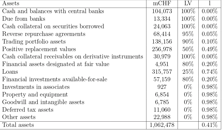
From table 3, it is seen that the liquidity spread ranges from 0bp (for e.g. cash) to 98bp for illiquid assets. This variation is somewhat larger than for Barclays. The reason is that the estimated severity of the LSE is larger with 25%. The average spread lav = 0.41% times the total assets gives 4.4b CHF, which is the total compensation required for liquidity risk per annum. This amount was a significant part (approx. 16%) of the net operating income of 28b in 2014.
Assets mCHF LV l Cash and balances with central banks 104,073 100% 0.00% Due from banks 13,334 100% 0.00% Cash collateral on securities borrowed 24,063 100% 0.00% Reverse repurchase agreements 68,414 95% 0.05% Trading portfolio assets 138,156 90% 0.10% Positive replacement values 256,978 50% 0.49% Cash collateral receivables on derivative instruments 30,979 100% 0.00% Financial assets designated at fair value 4,951 80% 0.20%
Loans 315,757 25% 0.74%
[image:19.595.105.528.129.377.2]Financial investments available-for-sale 57,159 80% 0.20% Investments in associates 927 0% 0.98% Property and equipment 6,854 0% 0.98% Goodwill and intangible assets 6,785 0% 0.98% Deferred tax assets 11,060 0% 0.98% Other assets 22,988 0% 0.98% Total assets 1,062,478 0.41%
Table 3: Liquidity spreads for the assets on UBS balance sheet.
6
Summary
This paper develops a liquidity risk valuation framework. The framework implies that liquidity risk of a bank affects the economic value of its assets. The starting observation is that the bank needs to liquidate some of its assets in an LSE, which means these will be sold at a discount. To develop the valuation framework, a liquidation strategy of the bank needs to be determined. It is shown that the optimal liquidation strategy suitable for valuation is a strategy where of each asset the same fraction is liquidated. The result is that cash flows are discounted including a liquidity spread. This liquidity spread consists of three factors: the probability of an LSE, the severity of an LSE, and the asset-specific discount in case of a liquidation in an LSE.
Acknowledgements
References
[Acharya & Pedersen(2005)] V. Acharyay and L. Pedersen (2005) Asset Pricing with Liquidity RiskJournal of Financial Economics77, 375-410.
[Amihud et al.(2005)] Y. Amihud, H. Mendelson and L. Pedersen (2005) Liquidity and Asset PricesFoundations and Trends in Finance1, 269.
[Amihud & Mendelson(1986)] Y. Amihud and H. Mendelson (1986) Asset pricing and the bid-ask spreadJournal of Financial Economics 17, 223-249.
[Barclays FY Results(2014)] Barclays (2014), Barclays 2014 Results Tables FY, ”http://www.barclays.com/barclays-investor-relations/results-and-reports/results.html” .
[BCBS(2010)] Basel Committee on Banking Supervision (2010) Basel III: Interna-tional framework for liquidity risk measurement, standards and monitoring.
[BIS(2008)] Bank for International Settlements (2008) Principles for sound liquid-ity risk management and supervision.
[Burgard & Kjaer(2011)] C. Burgard and M. Kjaer (2011) Partial differential equation representations of derivatives with bilateral counterparty risk and funding costs,The Journal of Credit Risk7, 75-93.
[Burgard & Kjaer(2013] C. Burgard and M. Kjaer (2013) Funding costs, funding strategies Risk Dec 2013, 82-87.
[Contet al.(2012)] R. Cont, A. Kukanov, and S. Stoikov (2012) The price impact of order book events,Journal of Financial Econometrics12(1), 47-88 [Grant(2011)] J. Grant (2011) Liquidity transfer pricing: a guide to better
prac-tice, BIS occasional paper No 10.
[Nauta(2015)] B. J. Nauta (2015) Liquidity Risk, instead of Funding Costs, leads to a Valuation Adjustment for Derivatives and other Assets, International Journal of Applied and Theoretical Finance18.
[Nauta(2013)] B. J. Nauta (2013) FVA and Liquidity Risk, Available at SSRN: http://ssrn.com/abstract=2373147.
[Obizhaeva(2008)] A. Obizhaeva (2008) The study of price impact and effective spread, Available at SSRN: http://ssrn.com/abstract=1178722.
![Table 1: Barclays balance sheet per 31 dec 2014 [Barclays FY Results(2014)].](https://thumb-us.123doks.com/thumbv2/123dok_us/7771073.717213/17.595.109.509.130.392/table-barclays-balance-sheet-dec-barclays-fy-results.webp)