Monetary policy options for mitigating the impact of the global financial crisis on emerging market economies

Munich Personal RePEc Archive

Monetary policy options for mitigating

the impact of the global financial crisis

on emerging market economies.

Dąbrowski, Marek A. and Śmiech, Sławomir and Papież,

Monika

Cracow University of Economics, Department of Macroeconomics,

Cracow University of Economics, Department of Statistics, Cracow

University of Economics, Department of Statistics

24 February 2013

Online at

https://mpra.ub.uni-muenchen.de/56337/

Monetary policy options for mitigating the impact of the global financial

crisis on emerging market economies

Marek A. Dąbrowski1_{, Sławomir Śmiech}2_{, Monika Papież}3

1_{Marek A. Dąbrowski: Cracow University of Economics, Department of Macroeconomics, Rakowicka 27,}

31-510 Cracow, Poland, marek.dabrowski@uek.krakow.pl (corresponding author)

2 _{Sławomir Śmiech: Cracow University of Economics, Department of Statistics, Rakowicka 27, 31-510 Cracow,}

Poland, smiechs@uek.krakow.pl

3 _{Monika Papież: Cracow University of Economics, Department of Statistics, Rakowicka 27, 31-510 Cracow,}

Poland, papiezm@uek.krakow.pl

Abstract

Though the hypothesis that exchange rate regimes fully predetermine monetary policy in the face of external shocks hardly finds any advocates on theoretical ground it has crept in the most of empirical research. This study adopts a more discerning empirical approach that looks at monetary policy tools used in order to accommodate the recent financial crisis. We investigated the GDP growth in 45 emerging market economies in the most intense phase of the crisis and found out that there is no clear difference in the growth performance between countries at the opposite poles of the exchange rate regime spectrum. Depreciation cum international reserve depletion outperforms the other policy options, especially the rise in the interest rate spread. We discovered certain complementarities between the information on the policy option and on exchange rate regime. Taking into account non-Gaussian settings, we decided to use quantile regression, which provide in addition, more complete picture of relationship between the covariates and the distribution of the GDP growth.

Keywords: Global financial crisis, Emerging market economies, Monetary policy, Exchange rate regime, Quantile regressions

JEL Classification: C21, E52, F31, F41

Introduction

One of the most important arguments against a fixed exchange rate regime is the

necessity of making the stabilization of an exchange rate a primary objective of monetary policy. By doing this, monetary authorities lose the autonomy in a sense that monetary policy

cannot be used in order to stabilize the output or employment (domestic objectives). The reasoning is rooted in the so-called trilemma or the impossible macroeconomic trinity: one cannot have the exchange rate stability, unfettered capital flows and monetary policy oriented toward domestic objectives at the same time2. The opponents of flexible exchange rates argue that such an arrangement contributes to uncertainty, which has an adverse effect on international trade and welfare.

Both these arguments were succinctly and vividly reported by Bordo and Flandreau (2003) as the “policy view” and “transactions costs” view on the links between integration

1 _{First version: February 24, 2013.}

2 _{For a traditional approach to the trilemma see Mundell (1963) and Fleming (1962). For the modern approach}

and exchange rate regimes. According to the former, flexible exchange rates foster the international adjustment process under nominal rigidities and imperfect factor mobility. The latter treats the exchange rate flexibility as a source of “a risk that cannot be diversified away and thus tantamount to a distortion preventing full specialization”3_.

Frenkel (1999) aptly pointed out that, even in the face of a gradual process of international financial integration, the trilemma does not mean that a country has to choose between the exchange rate stability and monetary autonomy: “there is nothing in the existing theory, for example, that prevents a country from pursuing a managed float under which half of every fluctuation in the demand for its currency is accommodated by intervention and half is reflected in the exchange rate” (Frenkel, 1999). Taking his idea a step further, one can argue that thanks to an additional monetary policy instrument, i.e. foreign market intervention, it is possible to ease the conflict between domestic and external objectives. In other words, even if there are no barriers to capital flows, the exchange rate regime per se does not fully predetermine the stability of output and exchange rate.

The global financial crisis has entailed large economic and social costs but at the same time provided a unique opportunity (in a sense of a natural experiment) to investigate the effectiveness of monetary policy options adopted by emerging market economies in order to accommodate adverse external shocks. These economies were different not only in their relative crisis resilience, but also in the policy option chosen to neutralize the the impact of crisis4.

The purpose of the article is to look at policy options adopted by monetary authorities in emerging market countries and to investigate their role in making the global financial crisis milder for their economies. The existing studies devoted to the role of monetary factors in shaping the relative crisis resilience have been focused on the type of exchange rate regime and not on the policy options actually adopted (e.g. see Berkmen et al., 2009, Blanchard et al.,

2010, Tsangarides, 2012)5. Our empirical strategy consisted of two complementary steps. Firstly, we looked for similarities in monetary authorities’ responses to the global financial crisis. The goal was to identify similar emerging market economies in terms of monetary policy tools used to accommodate external shocks. This stage of analysis was a missing link

3 _{The literature on a choice of exchange rate regime is ample. For a survey see Klein and Shambaugh (2010) or}

Rose (2011).

4 _{For a comprehensive study of emerging markets resilience during the global financial crisis see Didier et al.}

(2012).

5 _{For the sake of clarity, it ought to be emphasized that a lot of other explanatory variables, like the magnitude of}

between theoretical considerations and empirical research, and it was meant to serve as a substitute for the commonly used exchange rate regimes classification. Secondly, we looked for differences in the economic growth performance during the most intense phase of the crisis between the groups of emerging market economies. This stage was more in line with the

existing empirical literature, however, our approach was focused more on the effectiveness of alternative policy options oriented at crisis mitigation rather than on a sophisticated

comparison between countries that pegged their currencies with those that floated.

The paper is structured as follows. Section 2 reviews the literature on a role of exchange rate regime during the global financial crisis and elucidates our contribution. Section 3 outlines the two-step methodological approach adopted. The data and estimation results are presented in section 4, while Section 5 provides concluding remarks.

2. Exchange rate regimes and the crisis

Ghosh et al. (2010) divided the theoretical literature on the choice of exchange rate regime into three main categories. The first one is focused on the insulating properties of the regimes, constraints they put on macroeconomic stabilization policies, and their role in the adjustment processes. The second category investigates the benefits of monetary integration in the form of fostering deeper goods and capital markets integration and costs of losing monetary policy as an adjustment tool. The third one is related to a debate on an optimal stabilization programme: a fixed exchange rate can be used as a precommitment device by a central bank trying to impair deeply rooted inflationary expectations and restoring confidence in the domestic currency.

Our paper contributes to the first category of the literature on the choice of exchange rate regime. There is no professional consensus on which exchange rate regime is more conducive in fostering growth during financial crises. For example, Cúrdia (2009, 2007) showed that a fixed exchange rate regime is inferior to other monetary policy rules (Taylor type rules and targeting rules, in which a central bank targets at inflation, output and exchange rate stability) unless nominal rigidities are low or foreign demand for domestic goods is highly flexible. Using a dynamic general equilibrium model, Céspedes et al. (2004) showed that flexible exchange rates do play a role of a real external shocks absorber even in the environment with financial imperfections and balance sheet effects. Therefore, they concluded their analysis that “flexible rates are not only Pareto superior to fixed rates, but socially optimal”.

depend on the type of a shock hitting an economy (real versus nominal), but also on the type of a distortion that plagues it (goods markets versus asset markets frictions). They showed that under the assumptions of asset markets frictions and flexible prices, the famous “Mundell -Fleming‘s dictum” is turned on its head, i.e. flexible exchange rate regime is superior if monetary shocks prevail and hard peg is optimal if an economy is hit mainly by real shocks. Their conclusion is, therefore, that the usefulness of exchange rate fluctuations in absorbing

shocks hitting the economy is an empirical issue6.

Policy options for emerging market economies during the recent crisis were analysed by Ghosh et al. (2009). Their overall conclusion was that “there is no one-size-fits-all prescription, and the appropriate policy mix depends on the particular circumstances in each country, including a number of trade-offs”. As far as monetary policy is concerned, they stressed the importance of the trade-off between the benefits of lower interest rates and a depreciated currency for propping up domestic activity and exports against the contractionary effects of currency depreciation on unhedged balance sheets. The size of desirable currency depreciation depends on such factors as initial overvaluation, the exchange rate regime, balance sheet effects and possible regional contagion and systemic implications.

The empirical evidence regarding the role of exchange rate regimes during the recent financial crisis is mixed. Berkmen et al. (2012) searched for an explanation of resilience diversity among emerging markets in four groups of factors: (i) trade linkages; (ii) financial linkages; (iii) underlying vulnerabilities and financial structure; and (iv) the overall policy framework. After examining a plethora of various variables and robustness tests, they identified four main variables that explained a substantial fraction of (unexpected) growth performance in emerging markets: leverage (defined as a ratio of domestic credit to domestic deposits), primary gap, short-term external debt and the exchange rate flexibility. On the one hand, they concluded that one of the three preliminary policy lessons from the global financial crisis was that “exchange rate flexibility proved important for emerging markets in dampening the impact of large shocks”7_{. And on the other hand, they pointed ut that “the}

benefits of exchange rate flexibility appear limited to moving from a peg toward a more flexible regime” and “distinguishing between crawls and floats does not improve the fit”. Since this variable was the only one that seemed to matter among alternative monetary policy indicators considered, one could conclude that monetary policy did not mattere during the

6 _{For a stochastic version of their model see Lahiri et al. (2007).}

7 _{The other two were that reliance on short-term debt was associated with higher vulnerability and that strong}

most adverse phase of the crisis.

A similar conclusion referring to the significance of an exchange rate regime was drawn by Blanchard et al. (2010). Firstly, using the de facto exchange rate regime classification adopted by the IMF, they divided their sample (29 emerging markets) into two

groups: peggers and floaters. Secondly, they checked for an impact of the exchange rate arrangement on the unexpected GDP growth over the last quarter of 2008 and the first quarter

of 2009. Their theoretical model was not unambiguous on that issue, as it implied that the GDP growth in a country that pegged its currency depended also on whether the Marshal-Lerner condition was satisfied, on the strength of the balance sheet effect, and on the policy tools used in order maintain the peg (the policy rate and reserve decumulation). After controlling for the size of a shock, they found out that the growth was on average 2.7 percentage points lower in a country with a fixed rate regime, but this difference was statistically insignificant.

A different empirical strategy was adopted by Tsangarides (2012) who focused on the changes in actual GDP growth in 2008-2009 relative to 2003-2007 in a sample of 50 emerging market economies. His main finding was that after controlling for the trade exposure and financial linkages the choice of exchange rate regime was not an important determinant of the growth performance of emerging market economies during the crisis. Peggers, however, were faring worse in the recovery period 2010-2011.

Hutchison et al. (2010) investigated the effects of monetary and fiscal policies on the GDP growth during earlier financial crises in developing and emerging market economies (83 “sudden stop” episodes in 66 countries over 1980-2003 were examined). They found out that contractionary monetary and fiscal policies during a sudden stop exacerbated its recessionary consequences. Moreover, discretionary fiscal expansion alleviated adverse effects of a crisis, but monetary expansion had no discernible effect. Although at the time of sudden stops

countries had relatively rigid exchange rates on average, the exchange rate regime, included as a control variable, had no statistically significant effect on output costs of a sudden stop.

effects the country was trying to avoid.8 We develop this argument further and argue that it is not the exchange rate regime per se that matters in the crisis resilience, but the specific set of policy tools used in order to mitigate the contractionary pressure. Though we do not deny the fact that the exchange rate regime can have a certain impact on the monetary policy tools used

to accommodate external shocks, it by no means fully predetermines the policy response. The well-known fear of floating syndrome (Calvo and Reinhart, 2002) or a more recently

identified fear of losing international reserves behaviour (Aizenman and Sun, 2012) should induce to caution in research on exchange rate regimes9. This, however, seems to be present in theoretical literature only, whereas empirical analyses are preformed as if the exchange rate regime fully predetermined the policy reactions. The hardly surprising consequence is that exchange rate regimes do not matter empirically in explaining the resilience to financial crises. Our study departs from such an approach and looks at the policy tools used in order to accommodate averse external shocks. The empirical approach adopted in this paper seems to be both more consistent with and viable in the light of the theoretical findings and more promising in empirical research. Thus, we developed and applied an empirical strategy that is consistent with theory and contributes to the explanation of diversity among emerging market economies’ resilience to the global financial crisis. Moreover, it allows to solve the puzzle of small, if any, significance of exchange rate regime for growth performance during the first phase of the crisis.

3. Methodology

Statistical methods of unsupervised classification were used to identify the actual monetary policy options for crisis mitigation. The groups of countries obtained were expected to include economies that adopted similar monetary policy options. It was assumed that although the number of groups is unknown a priori, it should be neither too small nor too

large. In the former case the within group heterogeneity would be unduly large, whereas in the latter case the regression analysis would become impossible. Under such conditions, it was expedient to use various tools to classify the countries and to compare their results. Clustering was conducted by means of hierarchical methods in which groups are created recursively by linking together the most similar objects (different forms of linkage and different measures of distance were taken into consideration). Other methods of division, i.e. k-means method and

8 _{A similar conclusion was drawn by Ghosh et al. (2009).}

9 _{See also Blanchard et al. (2010b) who stated that the central banks actions in the emerging market economies}

partitioning among medodois (PAM) method proposed by Kaufman and Rousseeuw (1990), were also used. In both cases, after making the initial decision about the desired number of groups, objects are allocated in such a way that the relevant criterion is met. For the k-means method the allocation of objects should minimize within-group variance. In a case of the PAM

method at each step of the analysis the representatives of groups (medoids) are selected, and then the remaining objects are allocated to the group which includes the closest medoid. This

method is more robust to outliers than the k-means method, because it minimizes a sum of dissimilarities instead of a sum of squared Euclidean distance. The final classification of objects is, therefore, the result of the comparison of the results of respective grouping algorithms.

To evaluate the effectiveness of policy options for crisis mitigation the magnitude of the unexpected decline in the GDP growth is used. Statistical inference about relations was carried out within a framework of quantile regression analysis proposed by Koenker and Bassett (1978). In order to present the concept of quantile regression and the method of parameters estimation let us consider the following linear regression model:

i i i x

y  '  for i1,...,n (1)

where yi is a dependent variable, x_i' 









  is a vector of unknown parameters of the model, and i are independent

stochastic variables with identical distribution.

Let ri ^  yi xi'^

   

 _{stand for residuals of the regression model (1). In case of}

classical regression the OLS estimator is obtained by such a choice of parameters that minimizes the conditional distribution of the expected value of the response variable, i.e.





E | . In the case of quantile regression parameters are chosen in such a way that

conditional quantiles of dependent variables q









For each quantile 0 1 such a vector of parameters () is obtained by minimizing the

following criterion:

   

 

 





0 

)

( ( )0

^ ^

) ( ) 1 ( )

( min

 

    

i i

r r

i

i r

r (2)

The result is the parametric quantile regression:

 

  _i

i i x

y  

^

where ^ ^₀,...., ^ _'

  

 

  



 

 _p is a vector of coefficients that depends on the quantile  , and

0 ) | ( i xi 

q_  . Parameters of the model can be interpreted as the marginal change in the  th

conditional quantile of Y associated with a unit change in appropriate covariate. Kroenker (2005) emphasizes that a quantile regression in comparison to an OLS regression attains a

higher robustness and enables natural interpretation.

4. Data and empirical results

4.1. Data description

Our sample covered 45 emerging market economies (see Table 1). There is no one commonly accepted definition of emerging market economies. Generally they include countries which have reached a certain minimum level of GDP, have exhibited a relatively high rate of growth of GDP, but have small and not very deep financial markets and are vulnerable to internal and external forces10. To a first approximation these criteria are met by middle income economies. Several high income countries, however, are also classified as emerging markets, e.g. MSCI Emerging Markets Index covers 21 countries out of which 4 are classified by the World Bank as high income economies. According to the World Bank classification based on GNI per capita in 2009, our sample consisted of 13 lower middle income economies, 19 upper middle income economies and 13 high income economies.

Table1

Countries in the sample.

Algeria Czech Republic Macedonia, FYR Serbia

Argentina Egypt Malaysia Singapore

Armenia Estonia Malta Slovenia

Bolivia Georgia Mexico South Africa

Bosnia & Herzegovina Hong Kong Moldova Thailand

Brazil Hungary Morocco Tunisia

Bulgaria India Pakistan Turkey

Chile Indonesia Peru Uruguay

China Israel Philippines Venezuela, Rep. Bol.

Colombia Korea, Republic of Poland

Croatia Latvia Romania

Cyprus Lithuania Russia

Countries that adopted the euro before 2009 were also included in the sample. Though, as members of the monetary union, they do not pursue independent monetary policies, their

10 _{See Pearson website for an interesting comment on the definition of emerging markets or the Economist for a}

felicitous and humorous statement that: “’Emerging markets’is a useful term precisely because it is imprecise…

performance under common policy conveys interesting information for non-EMU countries in Central Europe. Slovakia was excluded from the sample because it adopted the euro at the beginning of 2009, which resulted in a related structural change in a monetary framework.

In all our specifications the growth performance is measured as a difference between

forecast and actual GDP growth in 2009, hereafter referred to as a GDP forecast error (GDP_FE) or unexpected growth performance. It is supposed to measure macroeconomic

effects of the first phase of the crisis in emerging market economies. To construct this variable, we have used IMF’s GDP growth forecasts that were published in the spring 2008 edition of World Economic Outlook, that is before the most intensive phase of the crisis started (IMF, 2008, 2012). With the variable of this kind it is easier to assess effectiveness of monetary policy options, which were used to mitigate the adverse impact of the crisis on an economy. It was these policies that were changed during the first phase of the crisis, thus the difference between projected and actual GDP growth remained in a relatively strong relation to the effectiveness of the policy option chosen. Another important factor that potentially contributed to that difference was the magnitude of an external economic shock and the economy’s vulnerability to such shocks. Some control variables, discussed below, were included in the regression to take care of the size of and vulnerability to external shocks.

Two other important arguments in favour of the chosen dependent variable are as follows. First, it automatically corrects for anticipated adjustments in growth, e.g. caused by the fact that different countries were in different phases of their business cycles. Second, as we used data on annual GDP growth in 2009, we allowed for differences in transmission of the global shocks to various economies11. Though Blanchard et al. (2010) also focused on the difference between the actual and forecast growth, they used the quarterly data. Their sample, however, covered barely 29 countries since the data of such frequency are not available for a large number of emerging market economies.

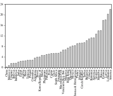
Data on unexpected GDP growth performance in emerging market economies in 2009 are depicted in Figure 1 (see also Table 3). The difference between forecast and actual growth was positive for all countries in the sample, but it was quite varied even for pairs of similar (not only in terms of the exchange rate regime) economies like Brazil and Mexico, Indonesia and Thailand or the Czech Republic and Poland. The difference ranged from less than 1 percentage point for China and Morocco to 18 percentage points or more for Baltic States and Armenia.

0 4 8 12 16 20 24 C hi na M or oc co U ru gu ay B ol iv ia In do ne si a In di a E gy pt A lg er ia Is ra el T un is ia Po la nd C ol om bi a A rg en ti na B ra zi l K or ea R ep ub li c of M al ta Ph il ip pi ne s Pa ki st an Pe ru C yp ru s C hi le So ut h A fr ic a Si ng ap or e M ac ed on ia FY R V en ez ue la R ep . B ol . M al ay si a H on g K on g T ha il an d M ex ic o B os ni a & H er ze go vi na T ur ke y H un ga ry C ze ch R ep ub li c Se rb ia B ul ga ri a C ro at ia R om an ia Sl ov en ia G eo rg ia M ol do va R us si a E st on ia L at vi a L it hu an ia A rm en ia GDP_FE

Fig. 1. Unexpected GDP growth performance in emerging market economies, 2009.

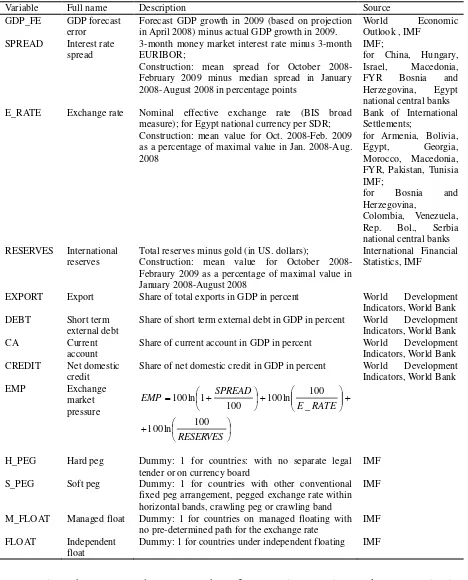
Three policy tools were used to extract policy options from the actual behaviour of monetary authorities: interest rate spread (SPREAD), exchange rate (E_RATE) and international reserves excluding gold (RESERVES). A detailed description of variables and sources is presented in Table 2. Since almost all central banks cut their policy rates during the crisis, we focused on the changes in difference between the domestic interest rate and the interest rate in the euro area12. Three-month money market interest rates were used. It was assumed that the degree to which the exchange rate was used was reflected in the magnitude of depreciation of domestic currency at the most intense phase of the crisis. To calculate the currency depreciation nominal effective exchange rates were used. The depletion of international reserves was treated as a variable describing the intensity of reserve utilisation to neutralize an external economic shock.

12 _{Three-month money market interest rates in all major advanced economies sharply decreased in the last}

Table 2

Variable description.

Variable Full name Description Source

GDP_FE GDP forecast error

Forecast GDP growth in 2009 (based on projection in April 2008) minus actual GDP growth in 2009.

World Economic

Outlook , IMF SPREAD Interest rate

spread

3-month money market interest rate minus 3-month EURIBOR;

Construction: mean spread for October 2008-February 2009 minus median spread in January 2008-August 2008 in percentage points

IMF;

for China, Hungary, Israel, Macedonia, FYR Bosnia and Herzegovina, Egypt national central banks E_RATE Exchange rate Nominal effective exchange rate (BIS broad

measure); for Egypt national currency per SDR; Construction: mean value for Oct. 2008-Feb. 2009 as a percentage of maximal value in Jan. 2008-Aug. 2008

Bank of International Settlements;

for Armenia, Bolivia, Egypt, Georgia, Morocco, Macedonia, FYR, Pakistan, Tunisia IMF;

for Bosnia and Herzegovina,

Colombia, Venezuela, Rep. Bol., Serbia national central banks RESERVES International

reserves

Total reserves minus gold (in US. dollars);

Construction: mean value for October 2008-Febraury 2009 as a percentage of maximal value in January 2008-August 2008

International Financial Statistics, IMF

EXPORT Export Share of total exports in GDP in percent World Development Indicators, World Bank

DEBT Short term

external debt

Share of short term external debt in GDP in percent World Development Indicators, World Bank

CA Current

account

Share of current account in GDP in percent World Development Indicators, World Bank CREDIT Net domestic

credit

Share of net domestic credit in GDP in percent World Development Indicators, World Bank

EMP Exchange

market pressure                        RESERVES RATE E SPREAD EMP 100 ln 100 _ 100 ln 100 100 1 ln 100

H_PEG Hard peg Dummy: 1 for countries: with no separate legal tender or on currency board

IMF

S_PEG Soft peg Dummy: 1 for countries with other conventional fixed peg arrangement, pegged exchange rate within horizontal bands, crawling peg or crawling band

IMF

M_FLOAT Managed float Dummy: 1 for countries on managed floating with no pre-determined path for the exchange rate

IMF

FLOAT Independent float

Dummy: 1 for countries under independent floating IMF

cent of GDP): export volume (EXPORT), short term external debt (DEBT), current account (CA) and net domestic credit (CREDIT). A detailed description of variables is provided in Table 2. Since these variables were supposed to reflect crisis vulnerability of an economy, we used their values at the end of 2007 (an additional advantage is that we avoided potential

endogenity problems). The more important the exports in a given economy, the more it is exposed to disturbances coming from the world economy (trade shocks). Both short-term external debt and current account deficit can be treated as proxies for economy’s dependence on the inflow of foreign capital. The greater they are, the more the economy is susceptible to financial shocks. Net domestic credit, which is the sum of financial sector’s claims both on the central government and other sectors of domestic economy, was used to take care of countries’ variation with respect to internal balance.

The size of an external shock was proxied by an additional control variable, i.e. a simple index of exchange market pressure, (EMP)13 (Table 2). One can reasonably expect that the economies exposed to more intense shocks experienced more pronounced decline in the economic growth and the attempt to assign this effect to any monetary policy option would be incorrect.

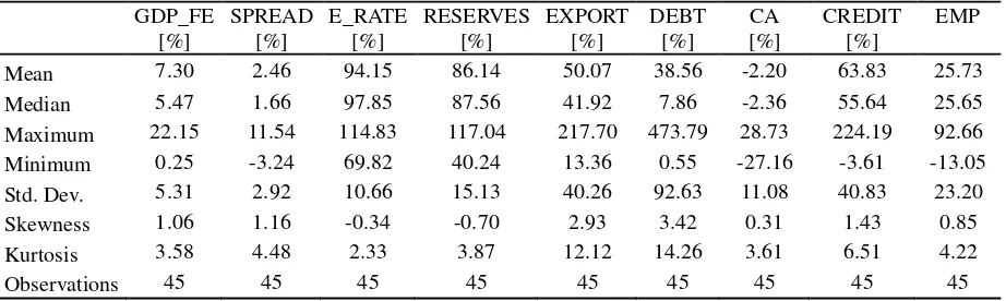
Table 3

Variables: descriptive statistics.

GDP_FE [%]

SPREAD [%]

E_RATE [%]

RESERVES [%]

EXPORT [%]

DEBT [%]

CA [%]

CREDIT [%]

EMP

Mean 7.30 2.46 94.15 86.14 50.07 38.56 -2.20 63.83 25.73

Median 5.47 1.66 97.85 87.56 41.92 7.86 -2.36 55.64 25.65

Maximum 22.15 11.54 114.83 117.04 217.70 473.79 28.73 224.19 92.66

Minimum 0.25 -3.24 69.82 40.24 13.36 0.55 -27.16 -3.61 -13.05

Std. Dev. 5.31 2.92 10.66 15.13 40.26 92.63 11.08 40.83 23.20

Skewness 1.06 1.16 -0.34 -0.70 2.93 3.42 0.31 1.43 0.85

Kurtosis 3.58 4.48 2.33 3.87 12.12 14.26 3.61 6.51 4.22

Observations 45 45 45 45 45 45 45 45 45

A set of dummies for de facto exchange rate arrangements were included in the regression analysis. To that end the IMF classification was used (IMF, 2009). It reports the actual exchange rate regimes at the end of April of 2008, that is before the most intense phase of the crisis. Exchange rate regimes were divided into four types (the IMF’s categories included in a respective type are given in brackets): hard peg arrangement (no separate legal tender, currency board) (H_PEG), soft peg arrangement (other conventional fixed peg, pegged

13 _{For more on this index and problems involved in its construction see Klassen and Jager (2011) and Li et al.}

exchange rate within horizontal bands, crawling peg, crawling band) (S_PEG), managed floating (manager floating with no predetermined path for the exchange rate) (M_FLOAT) and freely floating (independently floating) (FLOAT) (Table 2). Table 3 presents the descriptive statistics for the dependent and independent variables.

4.2. Monetary policy options and country groups

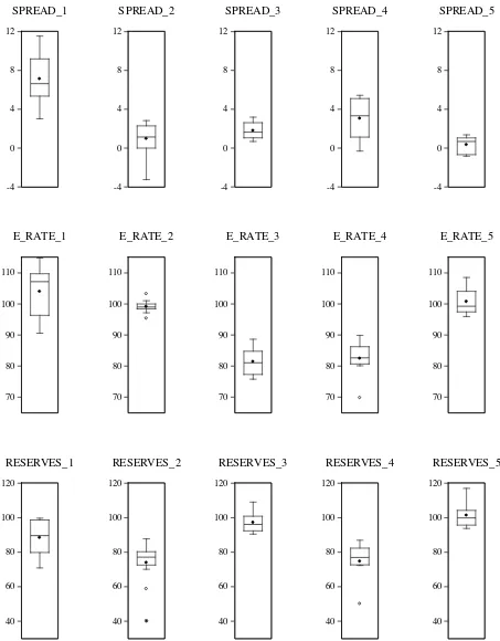
The objective of this part of the analysis was to uncover the similarities between countries with respect to monetary policy tools used in order to mitigate the effects of the crisis. Groups were identified by comparing three variables: nominal effective exchange rate (E_RATE), interest rate spread (SPREAD), and international reserves (RESERVES). Since RESERVES have greater variability (see Table 3) and, therefore, greater discriminatory power than the other two variables, all variables were standardized.

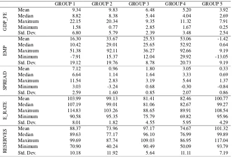
Groups of countries were determined with the use of hierarchical methods (Ward linkage, Euclidean distance), the k-means method and partitioning around medoids (PAM) method. All of them yielded very similar structures of groups of countries under the assumption that five groups are to be identified: either the composition of groups was the same or differences were observed for several objects only (4 or 5 countries). For countries which were not unambiguously classified, i.e. Armenia, Korea, Poland, the Czech Republic and Russia, the division based on the traditional hierarchical method was treated as conclusive. The reason for this was the assumption that such a classification of these five countries fitted well the regional composition of respective groups. Moreover, the size of respective groups was the most similar under this method of division. The final division into five groups of countries is presented in Table 4.

In spite of the relatively clear-cut results of the division into groups, it should be noticed that the groups identified were not strongly homogeneous. This can be seen in Figure

across country groups are presented in Figures 3 and 4 respectively.

Table 4

Country groups.

GROUP 1 GROUP 2 GROUP 3 GROUP 4 GROUP 5

8 13 9 7 8

Argentina Bosnia &

Herzegovina Brazil India Algeria

Armenia Bulgaria Chile Indonesia China

Bolivia Cyprus Colombia Korea, Republic of Egypt

Croatia Estonia Czech Republic Pakistan Hong Kong

Moldova Georgia Hungary Poland Israel

Russia Latvia Mexico Romania Singapore

Uruguay Lithuania Philippines Serbia Thailand

Venezuela Macedonia, FYR Turkey Tunisia

Malaysia South Africa

Morocco Malta

Peru Slovenia

Table 5

Descriptive statistics across country groups.

GROUP 1 GROUP 2 GROUP 3 GROUP 4 GROUP 5

GDP_

FE

Mean 9.34 9.83 6.48 5.20 3.92

Median 8.82 8.38 5.44 4.04 2.69

Maximum 22.15 20.34 9.35 11.32 7.91

Minimum 1.58 0.77 2.85 1.67 0.25

Std. Dev. 6.80 5.79 2.39 3.48 2.54

EMP

Mean 16.30 33.67 25.53 53.06 -1.42

Median 10.42 29.01 25.65 52.92 0.64

Maximum 51.38 92.11 36.27 92.66 9.19

Minimum -7.91 15.37 12.04 29.92 -13.05

Std. Dev. 19.12 19.76 8.78 20.73 9.19

SP

R

E

A

D Mean _Median 7.12 _6.64 0.96 _1.14 1.80 _1.64 3.05 _3.33 0.33 _0.69

Maximum 11.54 2.83 3.19 5.44 1.37

Minimum 3.03 -3.24 0.68 -0.30 -0.84

Std. Dev. 2.59 1.60 0.85 2.07 0.86

E

_

R

A

T

E Mean _Median 103.99 _107.19 99.13 _99.01 81.41 _81.06 82.46 _82.67 100.77 _99.27

Maximum 114.83 103.26 88.65 89.91 108.54

Minimum 90.58 95.35 75.79 69.82 95.96

Std. Dev. 8.01 1.82 4.55 5.95 4.29

R

E

SE

R

VE

S Mean 88.37 73.96 97.17 74.67 101.32

Median 89.63 77.17 96.10 76.99 99.89

Maximum 99.69 87.74 109.03 86.95 117.04

Minimum 70.90 40.24 90.49 50.09 93.79

-4 0 4 8 12 SPREAD_1 -4 0 4 8 12 SPREAD_2 -4 0 4 8 12 SPREAD_3 -4 0 4 8 12 SPREAD_4 -4 0 4 8 12 SPREAD_5 70 80 90 100 110 E_RATE_1 70 80 90 100 110 E_RATE_2 70 80 90 100 110 E_RATE_3 70 80 90 100 110 E_RATE_4 70 80 90 100 110 E_RATE_5 40 60 80 100 120 RESERVES_1 40 60 80 100 120 RESERVES_2 40 60 80 100 120 RESERVES_3 40 60 80 100 120 RESERVES_4 40 60 80 100 120 RESERVES_5

0 5 10 15 20 25

GDP_FE_1

0 5 10 15 20 25

GDP_FE_2

0 5 10 15 20 25

GDP_FE_3

0 5 10 15 20 25

GDP_FE_4

0 5 10 15 20 25

GDP_FE_5

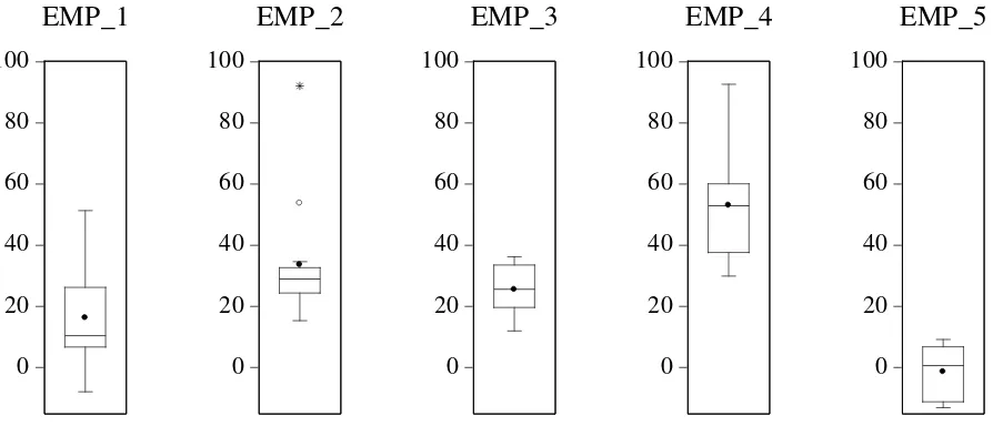
Fig. 3. Box plot of GDP growth loss (GDP_FE) across groups of countries.

0 20 40 60 80 100

EMP_1

0 20 40 60 80 100

EMP_2

0 20 40 60 80 100

EMP_3

0 20 40 60 80 100

EMP_4

0 20 40 60 80 100

EMP_5

Fig. 4. Box plot of exchange market pressure (EMP) across groups of countries.

A distinctive feature of the first group of countries (Table 4) was a relative increase of interest rate spread, a small depletion of international reserves and simultaneous stability of an exchange rate (in fact, on average a slight appreciation took place). This group includes countries under soft peg (Argentina, Bolivia, Croatia, and Russia) or managed float (others), i.e. exchange rate regimes that are called intermediate regimes (see Figure 2 and Table 5).

Countries in the second group (Table 4) used their international reserves to make the adjustment to external shocks less costly in terms of output (Figure 2). While this line of defence was characteristic mainly for countries under hard peg arrangement, two economies with soft peg (Morocco, Macedonia, FYR) and three under managed float (Georgia, Malaysia, Peru) were also included in this group.

(Colombia). One can intuitively expect them to allow for depreciation of their currencies and this intuition turns out to be correct. At the same time, they were reluctant to use their international reserves. Using the result from Aizenman and Sun (2012), one can conclude that monetary authorities in these countries revealed the “fear of losing international reserves”, which was stronger than the “fear of floating”. Interestingly, as many as six countries in this group (Chile, Colombia, Czech Republic, Mexico, Philippines, and South Africa) out of nine

were also included by Aizenman and Sun (2012) in their group of countries reluctant to allow for reserves depletion14.

A common feature of countries in the fourth group (Table 4) was the policy of reserves depletion and depreciation of domestic currency (Figure 2). This group was dominated by economies under managed float, but it also contained two independent floaters (Korea and Poland). Four countries included in this group (Indonesia, India, Korea and Poland) were qualified by Aizenman and Sun (2012) into their group of countries that were not reluctant to depreciate their currencies15.

The last group identified comprised of economies that experienced relatively weak external shocks. The exchange market pressure index was by a wide margin the lowest for this group with its median value close to zero and small variability (Figure 4 and Table 5). Monetary authorities in these countries were not forced to accommodate adverse external shocks with monetary policy tools: interest rate spreads hardly changed, depreciation was absent or its magnitude was limited, and there was no international reserves depletion; in fact in several economies reserves even went up and some currencies slightly appreciated. The GDP growth loss was on average the lowest in this group (Figure 4). It was a relative weakness of external shocks experienced by the countries in this group that contributed to a better GDP growth performance (Table 5)16.

14 _{The other three: Brazil, Hungary and Turkey were either classified as countries with depreciated currencies or}

absent in Aizenman and Sun’s sample. Differences can partly be explained by different methodologies:

Aizenman and Sun (2012) assumed a threshold level for reserves depletion (10 per cent), whereas in this study we use statistical methods to identify country groups. These differences partly result from the sample size:

Aizenman and Sun’s sample covered 21 emerging markets, whereas our sample is more than twice as numerous

as theirs.

15 _{The other three (Pakistan, Romania, Serbia) were absent in Aizenman and Sun’s sample.}

16 _{An additional factor that contributed to crisis mitigation was a relatively low degree of financial openness in}

4.3 Regression analyses

The magnitude of unexpected GDP growth loss was used to evaluate the effectiveness of monetary policy options for crisis mitigation that were identified in the previous subsection. To that end, alternative versions of quantile regression were constructed. Such a

regression allows to recover the complete picture of conditional distribution of dependent variable for every quantile and is robust to skewed tails and deviations from normality 17

Our benchmark regression model is given by equation (1). It relates the logarithm of unexpected decline in GDP growth in emerging market economies with control variables, exchange market pressure index, de facto exchange rate regime and groups identified in the first stage of our analysis.

j j Group

j gime

j j

Control

j CONTROL EMP REGIME GROUP

FE

GDP_ 0  2 Re  

ln (1)

where GDP_FEj stands for the GDP forecast error for country j, CONTROLj is a vector of

control variables (EXPORT, DEBT, CA, CREDIT) for country j, EMPj is an exchange

market pressure index for country j, REGIMEj is a vector of dummies for de facto exchange

rate regimes for country j, and GROUPj is a vector of dummies for groups for country j.

The analysis was divided into two complementary steps. First, various specification of

regression model (1) were analysed and compared. Thus, the impact of various vectors of explanatory variables on unexpected GDP growth performance was assessed. The objective of this part was to evaluate the sensitivity of regression models to changes in vector of explanatory variables and comparison of alternative specifications in terms of goodness of fit. The results of this part of analysis are presented for the median regression which is a special case of quantile regression. Next, we focused on the complete set of explanatory variables in equation (1) and carried out the analysis of quantile regressions. The results of this part are presented for 0.05, 0.25, 0.50, 0.75, 0.95 quantiles of conditional distribution of the dependent variable, i.e. unexpected GDP growth. Using the bootstrap method 95 per cent confidence intervals for parameters were calculated. This allowed to assess whether the effect of explanatory variables is stable and significant at different points of the unexpected GDP growth conditional distribution.

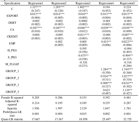
Regression results are summarized in Table 6. All regressions are based on variants of equation (1). Parameter estimates and their standard errors (given in parenthesis) are

17 _{Deviations from normality and skewness of distribution were characteristic for the residuals from the classical}

presented for median regressions18.

Table 6

Quantile-regression results (for median) using the logarithm of GDP forecast error as a dependent variable.

Specification Regression1 Regression2 Regression3 Regression4 Regression5

C 1.327***

(0.247)

1.285*** (0.320)

1.802*** (0.347)

0.194 (0.452)

0.224 (0.452)

EXPORT 0.013*** _(0.004) 0.014*** _(0.005) 0.010** _(0.005) 0.013*** _(0.004) 0.015*** _(0.004)

DEBT -0.002

(0.002)

-0.002 (0.002)

0.0002 (0.002)

-0.001 (0.002)

-0.003 (0.002)

CA -0.047*** _(0.010) -0.047*** _(0.010) -0.048*** _(0.012) -0.039*** _(0.010) -0.038*** _(0.009)

CREDIT -0.004

(0.003)

-0.005 (0.003)

-0.011*** (0.003)

-0.004 (0.003)

-0.007*** (0.002)

EMP _(0.005) 0.002 _(0.005) 0.005 0.013** _(0.006) 0.022*** _(0.006)

H_PEG 0.395

(0.356)

-0.094 (0.403)

S_PEG -0.675** _(0.258) -0.904** _(0.337)

M_FLOAT -0.326

(0.233)

-0.316 (0.266)

GROUP_1 1.284*** _(0.358) 1.740*** _(0.368)

GROUP_2 0.924***

(0.311)

1.027*** (0.318)

GROUP_3 0.909*** _(0.327) 0.836*** _(0.302)

GROUP_5 0.623

(0.487)

1.110** (0.427)

Pseudo R-squared 0.285 0.286 0.333 0.392 0.481

Adjusted

R-squared 0.214 0.195 0.185 0.235 0.287

Sparsity 1.956 1.997 2.129 1.847 1.781

Prob(Quasi-LR

stat) 0.001 0.004 0.015 0.002 0.001

Quasi-LR statistic 17.667 17.367 18.958 25.697 32.725

Standard errors are in parentheses under each parameter estimate. Quantile regression standard errors are based on bootstrap with 1000 replications. The sparsity function is computed with a Kernel method. ***, **, and * indicate significance at the 1, 5, and 10 percent levels, respectively.

Our basic specification in Table 6 includes four control variables only and a constant (column 1). Ratios of exports to GDP and current account balance to GDP are both correctly signed and statistically significant. Thus, higher exposure to foreign trade and greater dependence on foreign capital (more negative current account) result in a greater reduction in

unexpected economic growth. The other two controls are wrongly signed and insignificant. It is slightly surprising in a case of short-term external debt-to-GDP ratio that was statistically significant in other studies (e.g. Berkmen et al., 2012 or Blanchard et al., 2010). It is probably

18 _{Kernel (Epanechnikov) method was used to estimate sparsity function. The standard errors for the quantile}

because both current account balance and short-term external debt measure at least to some extent a similar thing, namely external vulnerability. Moreover, though Berkmen et al. (2012) did not include current account in their preferred specification, they admitted that “the current account balance is statistically significant even when the exchange rate regime or net open

position in foreign assets is controlled for, implying that while leverage was the crucial financial linkage, the degree of external imbalances was important”. The third reason is that

we adopted a different estimation technique. The variability of net domestic credit among countries seems to have negligible effect, both statistically and economically, on their growth performance.

Adding exchange market pressure index to the regression does not change the results significantly (column 2). Though the EMP had a positive impact on unexpected growth decline as expected, the effect was very weak.

The results of a regression that includes dummies for de facto exchange rate regime are presented in column 3. The relevant parameters should be interpreted in terms of a difference between a given exchange rate regime and a free floating which is treated as a reference regime.

The effect of exchange rate regime on GDP growth performance during the crisis seems to be quite weak for countries in the sample. Performance of economies with managed float or hard peg did not diverge from that of floaters at any conventionally adopted statistical significance levels. Only for countries under soft peg the growth decline was relatively weaker, although from the economic point of view this advantage was not large. Its magnitude can be illustrated with the following experiment19: were Poland under a soft peg arrangement, instead of a free float, at the time of the crisis, then ceteris paribus economic growth would be greater by 1.4 percentage point. It is interesting to observe that our general conclusion that the relation between exchange rate regime and growth performance is relatively weak is in

accordance with the empirical literature, e.g. Berkmen et al. (2012) also found that the benefits of exchange rate flexibility seem to be limited.

Regression with dummies for groups of countries identified in the previous step of our empirical strategy looks more revealing (column 4). There are dummies for each group of countries except for the fourth group, which is treated as a reference group. Differences with respect to that group are significant both statistically and economically, and the only exceptions are the fourth and fifth groups. Again, to illustrate the differences between groups

19 _{The results of an analysis of that type should not be interpreted in terms of a forecast. They are only supposed}

one can carry out a familiar experiment of moving Poland from the reference group to other groups and check for the effects20. Therefore, were Poland shifted to the group of countries that allowed for an increase in the interest rate spread (the first group), the GDP growth would fall 7.4 percentage points. If the “target group” was either countries that used their international reserves (the second group) or countries that depreciated their currencies (the third group), the economic growth would deteriorate by 4.3 and 4.2 percentage points

respectively. It is worth emphasizing that the last group (the fifth group) was characterized by a relatively low exchange market pressure. Since the EMP index was included in the regression as a control variable, a certain portion of an identity of the fifth group was probably seized by the EMP parameter. Regression without the EMP index looks slightly different: instead of an additional growth loss of 2.4 percentage point, Poland would earn 1.1 percentage points when shifted from the fourth group to the fifth one. The differences between other groups, however, were not statistically significant at 5 per cent level, which leaves some room for exchange rate regimes as explanatory variables21.

Regression with country groups has an advantage over regression based on de facto classification of exchange rate regimes not only on economic ground but also from a statistical point of view. An important feature of a model with groups of countries is the statistical significance of dummies for groups. Thus, information on similarities between countries as to the monetary policy options for crisis mitigation was important to explain variability of the differences between projected and actual GDP growth. Moreover, higher R-squared and adjusted R-R-squared for the regression with country groups than the one with exchange rate regimes lend some support for the former.

A more thorough picture of monetary policy options for crisis mitigation used by emerging market economies can be recovered from the regression that includes both exchange rate regimes and groups of countries (column 5). Two key conclusions can be drawn from the

regression like this. First, no set of variables makes information conveyed by the other statistically insignificant. A plausible interpretation is that information on exchange rate regime is complementary to and not substitutionary for information on groups of countries identified.

Second, while economic significance of coefficients for dummies for exchange rate regimes remained essentially unchanged (the results of the experiment with a change of

20 _{See the reservation in footnote 19.}

21 _{In order to check the differences between other groups' regressions were run. Each time a different group was}

exchange rate regime in Poland do not differ from those based on regression in column 3 by more than 0.3 percentage points22), coefficients that reflect differences between groups increased (the only exception is the coefficient for the third group, which virtually did not change). In other words, the inclusion of information on exchange rate regimes contributed to

an enhancement of differences between groups. For example, if Poland was to be moved to a group of countries that allowed for to a relative increase in the interest rate spread (the first

group), then ceteris paribus the GDP growth would collapse by as much as 13.7 percentage points. If the “target group” was countries that either lose international reserves (the second group) or accepted depreciation of their currencies (the third group), the growth loss would be 5.1 or 3.7 percentage points respectively. This time the difference between the fourth and fifth group turned out to be statistically significant: if Poland was moved to the fifth group, its GDP growth would be lower by about 5.7 percentage points23. Moreover, the differences between other groups turned out to be more palpable: out of a total of ten pairs of groups five were statistically different at 5 per cent level and one at 10 per cent level24. This result comes mainly from the pairs including the first group: for regressions excluding exchange rate regime dummies this group was not different from other groups (except for the fourth group), and, after including these dummies, the identity of the first group became sharper.

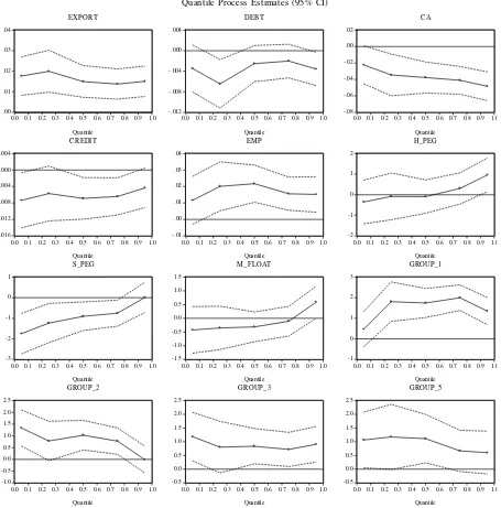
Parameter estimates of regression 5 are presented in more detail in Table 7 and Figure

5. Table 7 provides parameter estimates for quantiles  (0.05, 0.25, 0.5, 0.75, 0.95) with their standard errors, whereas Figure 5 depicts 95 per cent confidence intervals for parameter estimates. The results reveal that some variables, i.e. export to GDP ratio, EMP index, nest domestic credit and dummies for the third and fifth groups, have similar effect on unexpected GDP growth loss for any point of conditional distribution. This, however, is not the case with other variables. A given change in current account balance has the stronger impact on GDP growth performance, the higher the quantile of conditional distribution. The same holds for a dummy for the first group. For a dummy that identifies the second group the opposite conclusion holds: the higher the quantile of conditional distribution, the less evident the difference between the second group and the fourth group in terms of GDP growth loss. A similar conclusion holds for the dummy for soft peg: the reaction of a dependent variable becomes weaker as we move to the higher quantiles of conditional distribution. Parameters

22 _{For hard peg the difference is 1.6 p.p. but it is statistically insignificant.}

23 _{Such an adverse effect of this change is associated with the ceteris paribus reservation. Due to this}

assumption, the EMP index for Poland remains unchanged throughout the experiment. The characteristic feature of countries in the fifth group, however, is a low level of this index (see Figure 4).

24 _{Again detailed regression results are not presented here because of space constraint but are available upon}

for two other exchange rate regime dummies, i.e. hard peg and managed float, remain insignificant except for the last quantile. The same pattern holds for the external debt although its effect on GDP growth loss is also significant for 0.25 and 0.95 quantiles.

Table 7

Quantile regressions.

Specification Quantile 5 th Quantile 25th Quantile 50th Quantile 75th Quantile 95th

C -0.081

(0.640) -0.098 (0.661) 0.224 (0.451) 0.604 (0.446) 0.475 (0.473)

EXPORT 0.018*** _(0.005) 0.020*** _(0.005) 0.015*** _(0.004) 0.014*** _(0.004) 0.015*** _(0.004)

DEBT -0.003

(0.002) -0.006*** (0.002) -0.003 (0.002) -0.002 (0.002) -0.004* (0.002)

CA -0.022* _(0.012) -0.035** _(0.014) -0.038*** _(0.009) -0.041*** _(0.009) -0.048*** _(0.009)

CREDIT -0.007**

(0.003) -0.006* (0.003) -0.007*** (0.002) -0.006** (0.002) -0.004* (0.002)

EMP _(0.007) 0.012 0.020** _(0.008) 0.022*** _(0.006) 0.016*** _(0.005) 0.015** _(0.006)

H_PEG -0.352

(0.514) -0.085 (0.567) -0.094 (0.409) 0.302 (0.366) 0.963** (0.400)

S_PEG -1.752*** _(0.459) -1.237*** _(0.468) -0.904*** _(0.340) -0.755** _{(0.325) (0.368)} 0.014

M_FLOAT -0.425

(0.400) -0.353 (0.388) -0.316 (0.269) -0.109 (0.266) 0.588* (0.307)

GROUP_1 _(0.437) 0.464 1.803*** _(0.494) 1.740*** _(0.368) 1.996*** _(0.330) 1.343*** _(0.338)

GROUP_2 1.336***

(0.397) 0.782* (0.451) 1.027*** (0.318) 0.774** (0.303) -0.020 (0.281)

GROUP_3 1.184** _{(0.438) (0.462)} 0.803* 0.836*** _(0.302) 0.718** _(0.324) 0.907** _(0.337)

GROUP_5 1.064**

.00 .01 .02 .03 .04

0.0 0.1 0.2 0.3 0.4 0.5 0.6 0.7 0.8 0.9 1.0 Quantile EXPORT -.012 -.008 -.004 .000 .004

0.0 0.1 0.2 0.3 0.4 0.5 0.6 0.7 0.8 0.9 1.0 Quantile DEBT -.08 -.06 -.04 -.02 .00 .02

0.0 0.1 0.2 0.3 0.4 0.5 0.6 0.7 0.8 0.9 1.0 Quantile CA -.016 -.012 -.008 -.004 .000 .004

0.0 0.1 0.2 0.3 0.4 0.5 0.6 0.7 0.8 0.9 1.0 Quantile CREDIT -.01 .00 .01 .02 .03 .04

0.0 0.1 0.2 0.3 0.4 0.5 0.6 0.7 0.8 0.9 1.0 Quantile EMP -2 -1 0 1 2

0.0 0.1 0.2 0.3 0.4 0.5 0.6 0.7 0.8 0.9 1.0 Quantile H_PEG -3 -2 -1 0 1

0.0 0.1 0.2 0.3 0.4 0.5 0.6 0.7 0.8 0.9 1.0 Quantile S_PEG -1.5 -1.0 -0.5 0.0 0.5 1.0 1.5

0.0 0.1 0.2 0.3 0.4 0.5 0.6 0.7 0.8 0.9 1.0 Quantile M_FLOAT -1 0 1 2 3

0.0 0.1 0.2 0.3 0.4 0.5 0.6 0.7 0.8 0.9 1.0 Quantile GROUP_1 -1.0 -0.5 0.0 0.5 1.0 1.5 2.0 2.5

0.0 0.1 0.2 0.3 0.4 0.5 0.6 0.7 0.8 0.9 1.0 Quantile GROUP_2 -0.5 0.0 0.5 1.0 1.5 2.0 2.5

0.0 0.1 0.2 0.3 0.4 0.5 0.6 0.7 0.8 0.9 1.0 Quantile GROUP_3 -0.5 0.0 0.5 1.0 1.5 2.0 2.5

0.0 0.1 0.2 0.3 0.4 0.5 0.6 0.7 0.8 0.9 1.0 Quantile

GROUP_5 Quantile Process Estimates (95% CI)

Fig. 5. Quantile coefficients process.

5. Conclusions

Inconclusive empirical results on an effect of exchange rate regimes on a relative resilience of emerging market economies to the global financial crisis, indeed, should not be surprising. After all, macroeconomic theory does not imply that an exchange rate regime puts firm and strict binding constraints on macroeconomic policy. Neither does it fully predetermines which policy option of adjustment to an external economic shock will be chosen by monetary authorities.

of an external shock. Though this hypothesis hardly finds any advocates dealing with theoretical grounds, it has crept into numerous empirical researches. We depart from that line of empirical research and propose a more discerning approach that is based on an analysis of monetary policy tools used in order to accommodate external shocks.

The main conclusions are as follows. First, as predicted by macroeconomic theory, we found out that monetary authorities in countries under fixed exchange rates were more

reluctant to allow for depreciation of their currencies when the crisis hit than monetary authorities of floaters. There was, however, no clear (statistical) difference in the growth performance during the most intense phase of the crisis between countries at the opposite poles of exchange rate regime spectrum. Thus, second, it is not enough to look at exchange rate regimes when making comparisons between economies’ resilience to external shocks. Countries should be rather allocated to a given category according to the policy option used to mitigate the crisis. We constructed five such groups. After controlling for the size of a shock and external vulnerability, the option of depreciation cum international reserve depletion turned out to outperform the other policy options, i.e. either depreciation or reserve depletion, and, especially, the rise in the interest rate spread, which was the most costly line of defence.

Third, there are complementarities between information on group membership and on exchange rate regime adopted. Including the latter into the regression analysis allowed to sharpen the impact of groups on the growth performance. It is possible that there is something like a premium for consistency between the policy option chosen by monetary authorities and the prevailing exchange rate regime. This issue, however, requires a more extensive treatment, which we leave for future research.

Fourth, using quantile regressions, we were able to find out that our results are relevant not only for average but for almost all quantiles of conditional distribution of the dependent variable (GDP growth performance). This was especially pertinent to the impact of

policy options on growth: it was relatively stable with the exception of the extreme quantiles.

References

Aizenman, J., Chinn, M.D., Ito, H., 2010. The emerging global financial architecture: Tracing and evaluating new patterns of the trilemma configuration. Journal of International Money and Finance 29, 615-641.

Berkmen, S.P., Gelos, G., Rennhack, R., Walsh, J.P., 2012. The global financial crisis: Explaining cross-country differences in the output impact. Journal of International Money and Finance 31, 42-59.

Blanchard, O., Faruqee, H., Das, M., 2010. The initial impact of the crisis on emerging market countries. Brookings Papers on Economic Activity, Spring, 263–323.

Blanchard, O., Dell’Ariccia G., Mauro P., 2010b. Rethinking macroeconomic policy. Journal of Money, Credit and Banking 42 (Supplement s1), 199-215.

Bordo, M.D., Flandreau M., 2003. Core, Periphery, Exchange Rate Regime and Globalization” in: Bordo, M. D., Taylor, A., Williamson, J., (eds.) Globalization in Historical Perspective. Chicago University of Chicago Press, 417-468.

Calvo G.A., Reinhart, C.M., 2002. Fear of floating. Quarterly Journal of Economics CXVII (2), 379-408.

Céspedes, L.F., Chang, R., Velasco, A., 2004. Balance sheets and exchange rate policy. American Economic Review 94 (4), 1183-1193.

Chinn, M.D., Ito, H., 2008. A new measure of financial openness. Journal of Comparative Policy Analysis 10 (3), 309–322.

Cúrdia, V., 2007. Monetary policy under sudden stops. Federal Reserve Bank of New York Staff Report No. 278.

Cúrdia, V., 2009. Optimal monetary policy under sudden stops. Federal Reserve Bank of New York Staff Report No. 323.

Didier, T., Hevia, C., Schmukler, S.L., 2012. How resilient and countercyclical were emerging economies during the global financial crisis? Journal of International Money and Finance 31, 2052-2077.

Economist, 2012. It may no longer be wise to group these disparate countries together. Economist, April 21, 2012.

Fleming, J.M., 1962. Domestic financial policies under fixed and floating exchange rates. IMF Staff Papers 9, 369–379.

Frenkel, J.A., 1999. No single currency regime is right for all countries at all times. Essays in International Finance No. 215.

Ghosh, A.R., Chamon, M., Crowe, C., Kim, J.I., Ostry J.D., 2009. Coping with the crisis: Options for emerging market countries. International Monetary Fund Staff Position Note SPN/09/08.

Hutchison, M.M., Noy, I., Wang, L., 2010. Fiscal and monetary policies and the cost of sudden stops, Journal of International Money and Finance 29, 973-987.

IMF, April 2008. World Economic Outlook Database.

IMF, 2009. De facto classification of exchange rate regimes and monetary policy frameworks

as of April 30, 2008.

IMF, October 2012. World Economic Outlook Database.

Kaufman, L., Rousseeuw, P.J., 1990. Finding Groups in Data: An Introduction to Cluster Analysis, New York: Wiley & Sons.

Klassen, F., Jager, H., 2011. Definition-consistent measurement of the exchange market pressure. Journal of International Money and Finance 30, 74-95.

Klein. M.W., Shambaugh, J.C., 2010. Exchange rate regimes in the modern era. MIT Press, Cambride, MA – London.

Koenker, R., Basset, Jr., G., 1978. Quantile regression. Econometrica 46, 33–50. Koenker, R., 2005. Quantile Regression. Cambridge University Press.

Lahiri, A., Singh, R., Végh, C.A., 2008. Optimal exchange rate regimes: Turning Mundell-Fleming’s dictum on its head. In: Reinhart, C.M., Végh, C.A., Velasco, A. (Eds.), Money, crises, and transition. Essays in honor of Guillermo A. Calvo. The MIT Press, Cambridge, MA – London.

Lahiri, A., Végh, C.A., 2007. Output costs, currency crises, and interest rate defence of a peg. Economic Journal 117, 216-239.

Li, J., Rajan, R.S., Willett, T., 2006. Measuring currency crises using exchange market pressure indices: the imprecision of precision weights. Claremont Graduate University Working Paper No. 2006-09.

Mundell, R.A., 1963. Capital mobility and stabilization policy under fixed and flexible exchange rates. Canadian Journal of Economic and Political Science 29 (4), 475–485.

Obstfeld, M., Shambaugh, J.C., Taylor, A.M., 2010. Financial stability, trilemma, and international reserves. American Economic Journal: Macroeconomics 2 (2), 57-94. Obstfeld, M., Shambaugh, J.C., Taylor, A.M., 2005. The trilemma in history: Tradeoffs among

exchange rates, monetary policies, and capital mobility. Review of Economics and Statistics 87 (3), 423-438.

Pearson. Emerging markets defined. www.pearsoned.co.uk/

Rose, A.K., 2011. Exchange Rate Regimes in the Modern Era: Fixed, Floating, and Flaky. Journal of Economic Literature 49 (3), 652-672.

Gertler. M.J. (Eds.), International Dimensions of Monetary Policy. University of Chicago Press, Chicago and London.