Munich Personal RePEc Archive
Data-based priors for vector
autoregressions with drifting coefficients
Korobilis, Dimitris
January 2014
Online at
https://mpra.ub.uni-muenchen.de/53772/
Data-based priors for vector autoregressions
with drifting coefficients
Dimitris Korobilis
University of Glasgow
January 2014
Abstract
This paper proposes full-Bayes priors for time-varying parameter vector autoregressions (TVP-VARs) which are more robust and objective than exist-ing choices proposed in the literature. We formulate the priors in a way that they allow for straightforward posterior computation, they require minimal input by the user, and they result in shrinkage posterior representations, thus, making them appropriate for models of large dimensions. A comprehensive forecasting exercise involving TVP-VARs of different dimensions establishes the usefulness of the proposed approach.
Keywords: TVP-VAR, shrinkage, data-based prior, forecasting
JEL Classification: C11, C22, C32, C52, C53, C63, E17, E58
1
Introduction
During the early stages of the development of vector autoregressive (VAR) models for modelling and forecasting macroeconomic data (Sims, 1989; Littermann, 1979), it has been recognized that such multivariate time series models can be subject to “curse of dimensionality” problems. Coefficients tend to increase exponentially with the number of endogenous variables or the number of lags. Therefore, it is no surprise that the early VAR literature was exclusively Bayesian, since prior distributions can provide a straightforward basis for imposing data-based shrinkage towards zero of irrelevant coefficients. For macroeconomists who typically work with monthly or quarterly data, saving degrees of freedom seems to be recognized as an issue of paramount importance in order to obtain reliable inference and communicate accurate forecasts to policy-makers.
Nevertheless, despite the vast development of Bayesian computational and shrinkage methods since the late 1970s, the econometrics literature has only had a few developments on the shrinkage front. The traditional “Minnesota-prior”, an empirical-Bayes prior which is due to Littermann (1979) and co-authors (see, e.g. Doan, Litterman, and Sims, 1984), still dominates many applications of VAR models in economics. With the exception of the recent contribution of Giannone, Lenza and Primiceri (2012), selecting the infamous shrinkage factor of the Minnesota prior, i.e. the prior hyperparameter controlling shrinkage of the VAR coefficients, has been more of an art than exact science.
In this paper we develop a simple algorithm for selecting data-based priors for vector autoregressions with time-varying coefficients and stochastic volatility. We achieve this task by introducing full Bayes (hierarchical) priors which allow prior hyperparameters to be updated by the data using standard posterior expressions. Based on a simple reparametrization for state-space models (e.g. Frühwirth-Schnatter and Wagner, 2010; Belmonte, Koop and Korobilis, 2014) we show that we can develop simple prior structures which add minimal computational complexity to the standard TVP-VAR estimation algorithm used in the macroeconomic litera-ture (e.g. the popular algorithm used in Primiceri, 2005). We show that such data-based priors also have the property of shrinking time-varying VAR coefficients towards zero or towards time-invariance, in which case we can save valuable degrees of freedom for estimation and forecasting.
prior opinion about how much time-variation we may expect to find in all TVP-VAR coefficients usually breaks down to the choice of a single hyperparameter; see the detailed discussion in Primiceri (2005, Section 4.1). While such simplification makes prior selection easier and more convenient (only a single hyperparameter to select), there is a “downside risk” of following this approach in the flexible class of TVP-VAR models, since posterior quantities applied economists usually report (e.g. forecasts, impulse responses) can become very sensitive to selection of this hyperparameter1.
The purpose of this paper is not to criticize the previous empirical macro-economic literature; rather, its main intent is to propose a simple solution to an issue that can be daunting and confusing to the applied economist. The examples from the literature presented above show vividly that it is essential to establish methods for prior selection in TVP-VARs which allow a more automatic/default and robust determination of the prior structure, instead of relying solely on researchers’ beliefs and experience. At the same time, since TVP-VARs are very popular with researchers in central banks and elsewhere, it is quite important to be careful enough to develop a simple posterior estimation framework that can be useful and meaningful to applied economists. That is, estimation should be both robust to subjective prior beliefs and reproducible, helping applied economists to communicate reliable results to their clients, managers, or the public. In that respect, this paper presents very simple tweaks and modifications to the very popular TVP-VAR framework of Primiceri (2005), thus allowing users to shrink coefficients in a data-based manner. Posterior expressions are based on conjugate priors and are, thus, straightforward to derive. Note that computational simplicity is a priority in this paper, so that the Gibbs sampler is preferred compared to other potentially more powerfull and elegant Markov Chain Monte Carlo (MCMC) and Sequential Monte Carlo (SMC) algorithms for prior selection.
The most important aspect of the proposed Bayesian estimator is that it decides (based on information in the likelihood) which coefficients are time-varying or not, as well as which coefficients are zero or not; see Belmonte, Koop and Korobilis (2014), Eisenstat, Chan and Strachan (2013) and Groen, Paap, and Ravazzolo (2012) for similar approaches. In general shrinkage estimators add some more bias (compared to unbiased estimators such as OLS in an unrestricted, time-invariant VAR), in order to massively reduce the variance of the estimated coefficients. We show that in the case of TVP-VARs, this kind of variance-bias tradeoff results in dramatic improvement in model fit, and large gains in forecast accuracy even when we evaluate only mean forecast (and not the whole predictive distribution). In a forecasting exercise using TVP-VARs with four to seven variables2, we show
1Primiceri (2005) chooses this hyperparameter to be(0.01)2, Canova and Gambetti (2009) choose
a value of 0.0003, and Cogley and Sargent (2005) choose a value of 3.5e 4. As with the traditional Minnesota prior, selection of this shrinkage coefficient is an art and not an exact science.
2Note that, following the finindings of Clark and Ravazzolo (forthcoming), all TVP-VAR models
that improvement in forecast accuracy from shrinkage is massive even for the smaller four-variable systems. Additionally, confirming the results of D’Agostino, Gambetti and Giannone (2013) and Korobilis (2013c), forecasting gains from using time-varying instead of time-invariant VARs are substantial for “inherently nonlinear” variables such as GDP and inflation.
The next section serves as an introduction to the properties of time-varying pa-rameter VARs, the overparametrization problem, as well as a formal and intuitive explanation of the source of the numerical (in)stability issues that can occur in this model class. We subsequently present formally the simple modifications explained above, which result in a more stable and robust approach to esitmating TVP-VARs. In Section 3 we begin with an empirical demonstration of the robustness of data-based shrinkage priors, and conclude with a comprehensive forecasting exercise. In Section 4 we summarize the findings of this paper and reflect on the importance of the proposed econometric methods.
2
Methodology
2.1
Understanding time-varying parameters VARs
Let yt be a vector of n variables of interest for t = 1, ...,T. A p-lag time-varying coefficients VAR model foryt takes the following form
yt =ct+B1,tyt 1+...+Bp,tyt p+εt, (1) wherect is an 1 vector of intercepts,Bi,t,i =1, ..,p, are VAR coefficient matrices of dimensionsn n, andεt N(0,Ωt)are shocks withΩtann nheteroskedastic VAR covariance matrix. The purpose of this paper is to consider shrinkage of the “large” vector of VAR coefficientsBt = ct,B1,t, ...,Bp,t . Macroeconomic data are usually highly correlated and subject to abrupt changes in volatility, thus, we assume that there should not be any benefits from shrinking Ωt towards zero or
towards time-invariance; see for instance the discussion in Clark (2009) and Sims and Zha (2006). In light of this assumption we allow Ωt to follow the typical
multivariate stochastic volatility specification of the sort introduced in Primiceri (2005); exact specification details are provided in the appendix.
It is trivial to show that the VAR above can be written as a linear regression of the form
Y = X β + ε
whereY = (y1, ...,yT)0,B= (B10, ...,B0T)0,ε= (ε1, ...,εT)0and
X =
2 6 6 6 4
x1 0 0
0 x2 . .. ...
... ... ... 0
0 0 xT
3 7 7 7 5.
wherek = np+1 andxt =
h
1,y0t 1, ...,y0t pi0. In the formulation above the Tk Tkmatrix (X0X)is of rank T and is not invertible, meaning that likelihood-based estimation cannot be used here. To deal with this issue, the standard practice in the literature (at least since the time of Cooley, 1971) is to impose more structure in the model by assuming that the VAR coefficients evolve as multivariate random walks. Following the notation of Primiceri (2005) and many others, the full time-varying coefficients VAR takes the form
yt = z0tβt+εt (3)
βt = βt 1+ηt, (4)
where zt = In xt, and βt = c0t,vec B01,t
0
, ...,vec B01,t 0 0
subject to the
initial condition β0 N(b0,P0). In the equation above ηt N(0,Q) is a state disturbance term with system covariance matrix Q of dimensions m m,
m=k n. This is the typical specification of a time-varying parameter VAR which has been embraced so much in macroeconomics; see Doan, Littermann and Sims (1984) for a review. We can show that now the information in X is enough to estimateβt (which is now centered in βt) and the covariance matrix Q.
Nevertheless, an important econometric issue arises with such a specification. Using repeated substitution it is easy to show that equation (4) implies that
var(βt) = P0+tQ. This result reveals that even before observing the data, the
variance ofβt will tend to explode as t ! ∞, which is an obvious implication of
the random walk assumption in (4). Thus, macroeconomists tend to choose modest values for P0, and impose very tight priors on Q, thus regularizing the posterior
variance ofβt. A typical implementation of prior selection in such models is to fit a VAR in a training-sample, and use the posterior moments to elicit the priors for the TVP-VAR in the estimation sample (see Primiceri, 2005).
In practical situations, though, application of training sample priors is not optimal. For many short time series (e.g. Euro-Area data) a training or hold-out sample might not be an option. Additionally, whilst a training sample prior is a very informative and subjective prior, the researcher might fail to fully understand its features and its implication for estimating the amount of time variation in the VAR. The size of the training sample or other selected hyperparameters3 will
3See for example the hyperparameters relating to the prior ofQin Primiceri (2005, Section 4.1),
greatly affect posterior inference, so that most probably the researcher will have to set these ex-post (i.e. after observing the posterior) which implies a fair degree of data-minning. Lastly, the information in observed data might not be enough to estimate particular elements of βt, and the corresponding eigenvalues of the conditional variance var βtjyt . For example, some eignevalues of var βtjyt
can become too high in conflict with prior information or data history (Kulhavý and Zarrop, 1993); or as we add more lags in the VAR and k grows large it is expected that the sample eigenvalues of var βtjyt will diverge from the population eigenvalues (Stein, 1975).
2.2
A shrinkage representation of the TVP-VAR
In order to be able to specify data-based priors on the TVP-VAR which can provide shrinkage of coefficients, we first follow Belmonte, Koop and Korobilis (2013) and use the following reparametrization
yt = z0tα+z0tαt+εt, (5)
αt = αt 1+ηt, (6)
with initial conditionα0 N(0, 0 Im), i.e. a point mass at zero. This TVP-VAR
is observationally equivalent to the one presented in equations (3)-(4), where it holds that α β0 and αt = βt β0. The difference is that, roughly speaking, now the VAR is decomposed into a part which is a constant parameter VAR (z0tα) and a part which describes how much additional time-variation we can add to the constant parameter VAR (z0tαt). Therefore, an immediate advantage is that we can separately focus on the task of saving degrees of freedom by either shrinking the time-varying coefficientsαt, or the constant coefficientsα, or both.
The first step in our analysis is to allow the initial condition α β0 to be updated from the data. Therefore, one now can explicitly define full-Bayes priors forαbased on the Normal distribution, which are of the form
α N(0,V)
V = diag(τ1, ...,τm) (7)
τi F(c1,c2), i =1, ..,m
whereVis a diagonal prior variance with elementτi which has as a prior density
F with parameters c1 and c2. In the next subsection we follow Korobilis (2013) and explicitly define appropriate forms for the density F. Here it suffices to note that once theτi’s have their own prior then they will be updated from the data. Unlike standard practice where a common variance parameter (say τ such that
“large” then αi will have a fairly uninformative prior variance, however, if the posterior ofτiis concentrated at zero then the implied prior ofαiis approximately
N(0, 0) which implies that the posterior of αi will also be a point mass at zero. Therefore, we have a flexible situation where different elements ofαcan be shrunk (or not) with a varying degree, depending on the absolute value of eachτi.
The second step in our analysis is to update in a data-based manner (and also shrink) the time-varying part of the TVP-VAR, that is the coefficientαt. Notice that if the covariance matrix Q of αt is shrunk to zero, then the TVP-VAR is shrunk toward a constant parameter VAR, since from (6) we can infer that in this case
αt = αt 1 = ... = α0 and α0 N(0, 0 Im) 0. Therefore, shrinkage of Q towards zero also means shrinkage ofattowards zero for allt, which in turn results in shrinkage of the TVP-VAR towards a time-invariant VAR. It becomes obvious then that we need to specify a data-based prior for Q in the spirit of the prior presented in equation (7). However, while a conjugate prior forQis the inverse-Wishart distribution, there are no obvious hierarchical priors that can be used in this case. To be exact, Bouriga and Féron (2013), and references therein, do examine hierarchical shrinkage Wishart priors, nevertheless, their formulations are not conjugate and posterior computation can become demanding in high dimensions4. In contrast, in this paper we make the assumption that - in the spirit of the Minnesota prior tradition for constant parameter VARs - coefficients which are a-priori shrunk to zero based on the prior (7), should also be shrunk to time-invariance. Alternatively, coefficients which are important and initialized to a value different from zero are the most probable candidates for being time-varying. Additionally, coefficients on higher lags are less probable for being the main source of time-variation in a VAR. Here we consider two versions of this prior belief which - (ab)using terminology from the image processing literature - we termsoft thresholdingandhard thresholding, respectively. In soft thresholding we specify the prior
Q iW v,kQV , (8)
while in hard thresholding we further restrictQby assuming it is diagonal, that is, we use the prior
Qii iG v,kQVii , (9) for i = 1, ...,m. Both priors depend on the diagonal matrix V, which will be estimated by the data. The difference is that in equation (8) if a diagonal element
4An alternative way, which is quite attractive, is to use a reparametrization such as the one in
ofV happens to be zero, then the respective element of the posterior of Q won’t necessarily be exactly zero (but it might become small, i.e. shrunk). In the second prior, given that Qis diagonal, if Vii τi becomes zero then the posterior of Qii will also be zero. Therefore, the second prior can result in massive reduction in estimation error (variance of posterior), with the downside risk of a very large bias, while the first prior provides a more balanced tradeoff between bias and variance. For medium-sized TVP-VARs the soft thresholding prior can be a reasonable choice, while for TVP-VARs of very large dimensions (30+ variables) the hard thresholding prior might be needed. Notice that the researcher has to choose hyperparameters v,kQ5 for both priors for Q. In Section 3.1 we explain how to choose these hyperparameters, and we show using real data that estimation of the TVP-VAR is not that sensitive to their choice.
To summarize, we have presented a framework for updating the time-varying VAR coefficients using a prior whose hyperparameters are updated from the data. We implement this by using a simple decomposition of the time-varying coefficients into the time-invariant and the time-varying part. Then we apply standard conjugate analysis and simplify selection of the prior hyperparameters into selection of a diagonal prior covariance matrixV. According to equation (7)
Vhas its own prior distribution, reflecting our desire for this matrix to be updated by the data and, thus, admit a parametric posterior distribution of its own. In the next subsection we examine more carefully choices of distributions forV which have desirable properties in the context of VAR models.
2.3
Hyperprior distributions for VARs
In a univariate regression setting, Korobilis (2013a, 2013b) shows several possibili-ties for specifying hyperprior distributions based on a Normal conjugate prior. In our case we need to consider the fact that in a VAR model coefficients correspond to different equations and to lags of the dependent variables. In particular we use three types of hierarchical priors reflecting a varying degree of subjective beliefs about which coefficients should be shrunk. In the first case, we use a noninformative prior on each element τi, i = 1, ...,m, of the prior covariance matrix V = diag(τ1, ...,τm), in which case the data will update τi in a way where coefficients αi will be a priori equally likely to be shrunk to zero or not. In the second and third cases, we allow the degree of shrinkage to increase as the number of lags increase. That way we can prevent overfitting and preserve degrees of freedom, using this idea from the Minnesota-prior literature; see Litterman (1979). The difference in these two last formulations we propose is that in one we implement a simple variant where the discounting of distant lags is chosen
5For the reader familiar with the analysis of Primiceri (2005), k
Q is a crucial hyperparameter
subjectively from the researcher, while in the other the discounting of distant lags is more data-based.
Noninformative prior
The simplest prior choice forτiis to use a Jeffrey’s prior of the form
τi ∝ 1
τi. (10)
Minnesota-type prior with subjective choice
Here we use the following structure forτi
τi iG κ1,κ2 1
r2 , (11)
for lag lengths r = 1, ...,p. In this case autoregressive coefficients have prior varianceτiwhich is updated from an inverse Gamma distribution with prior scale parameter that discounts more distant lags quadratically. This discount factor of
1
r2,r=1, ...,p, is similar to the one used in the original Minnesota prior.
Objective Minnesota-type prior
In this case, we set τi = λ 1ξr 1 and we select separate priors for λ and ξr
wherer =1, ...,pindexes ther-th lag. Following Bhattacharya and Dunson (2011) the prior we define takes the form
τi = λ 1ξr 1 λ 1 G(v/2,v/2),
ξr =
∏
rl=1δl, (12)δ1 G(ρ1, 1),
δl G(ρ2, 1), l 2 .
In this case the “common” variance for all coefficients isλ. However, coefficients on lag k will have total variance λ=1ξr 1, where ξr = δ1δ2...δr is a multiplicative Gamma process. Under the conditionρ1 > 1 theξ
r’s are stochastically increasing as the number of lags increase, in which case the total prior variance τi will be decreasing with the lag length of the VAR. Instead of the fixed geometrical decrease of the prior scale in the traditional Minnesota prior, this prior allows each lag-length to be penalized with different intensity and not necessarily linearly or exponentially. Nevertheless, the prior in (12) can still be considered a Minnesota-type prior since still it is the case that more distant lags will have larger penalty a-priori.
3
Empirics
3.1
Understanding the effect of shrinkage priors
The first step in our analysis is to delve deeper into the exact effect of the priors presented above on estimation of the time-varying VAR coefficients by means of a real-data example. At this stage the interest does not lie on the exact prior distribution for V = diag(τ1, ...,τm), that is we are not interested to assess whether a noninformative, subjective Minnesota, or data-based Minnesota prior is better. This comparison is left as part of the empirical forecasting in the next subsection. Here our aim is to examine different patterns of shrinkage for the VAR coefficients βt by restricting its state covariance Q through the priors (8) and (9), respectively. For that reason, for the whole analysis presented in this subsection we are using a simple 3-variable TVP-VAR on inflation (growth rate on GDP deflator), unemployment rate, and three-month interest rate estimated over the period 1960Q1-2013Q2. The TVP-VAR has only two lags and an intercept, as well as multivariate stochastic volatility. Therefore, this is the typical New Keynesian system that Primiceri (2005) and others have considered in their analysis.
First, we estimate this simple TVP-VAR using a data-based prior forV6, and the soft thresholding onQ. Note thatQdepends on hyperparametersv, kQ which we need to choose, as well as the scale matrixV which is updated from the data. For the degrees of freedom hyperparametervwe set it tov=m+2, so that the inverse Wishart prior is a well-defined distribution with a finite mean and variance7. Therefore, a large part of the prior sensitivity in the TVP-VAR system is expected to originate from selection of the prior scale matrix ofkQV. In the case of Primiceri (2005) V is fixed to the OLS estimate from a constant parameter VAR in a pre-sample (training pre-sample), so that selection ofkQsolely determines prior sensitivity. In this paper,Vadapts in each MCMC iteration based on information from the data and is not fixed (it is a random variable with well-defined posterior distribution), therefore, selection ofkQ can be less harmful. Therefore our algorithm allows the prior scalekQVin priors (8) and (9) to adapt in such a way that the data will almost always determine their combined optimal value, even thoughkQ has to be chosen by the researcher.
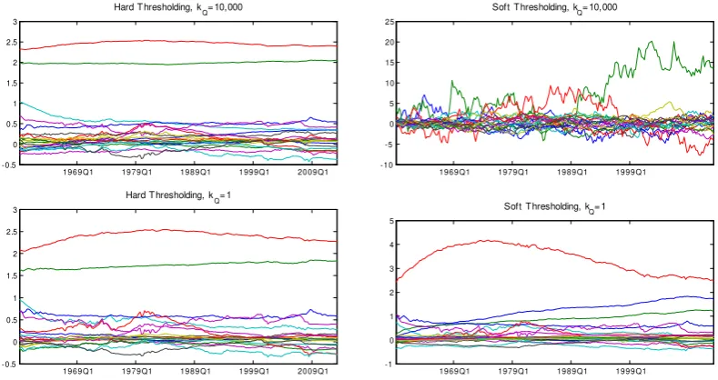
In order to demonstrate this case, we plot in Figure 1 the posterior means of βt = α +αt when using the hard thresholding (left panel) and the soft thresholding (right panel) priors forQfor two substantially different values of the hyperparameterkQ namely 10, 000 and 1. This is a very extreme example which
6In particular we use the noninformative hyper-prior in equation (10), however, we could have
come to the same conclusion by using priors (11) or (12).
7In the case of the hard thresholding prior, which is based on an inverse gamma distribution and
not an inverse wishart, we still use the same formula, that isv=1+2, since nowQiiis univariate.
This choice ensures that the prior mean and variance of this distribution exists (but we needv>3
is used to test the numerical stability of our algorithms. Posterior mean estimates based on the hard thresholding prior are strikingly similar, showing that this prior has minimal prior sensitivity. The soft thresholding prior, which assumes that Q is a full matrix with inverse Wishart prior, is considerably more sensitive to selection
kQ, however, it is numerically more stable than what would be expected under traditional priors: the reason why posterior mean estimates using the training sample prior are not plotted in Figure 1 is that estimation collapses in the case
kQ = 10, 000 (draws of Q become non-positive definite, because Q explodes, leading alsoβt to explode).
19 6 9 Q1 19 7 9 Q1 19 8 9 Q1 19 9 9 Q1 20 0 9 Q1 -0.5 0 0.5 1 1.5 2 2.5 3
Hard T hresholding, kQ= 1
19 6 9 Q1 19 7 9 Q1 19 8 9 Q1 19 9 9 Q1 20 0 9 Q1 -0.5 0 0.5 1 1.5 2 2.5 3
Hard T hresholding, kQ= 10,000
19 6 9 Q1 19 7 9 Q1 19 8 9 Q1 19 9 9 Q1 -10 -5 0 5 10 15 20 25
Soft T hresholding, kQ= 10,000
19 6 9 Q1 19 7 9 Q1 19 8 9 Q1 19 9 9 Q1 -1 0 1 2 3 4 5
[image:12.595.107.502.262.471.2]Soft T hresholding, kQ= 1
Figure 1. Posterior means of TVP-VAR(4) estimates from a typical three-variable system on prices, output and interest rate. The top panel shows coefficient
estimates whenkQ =10, 000 for the hard and soft thresholding priors, respectively. The bottom panel shows how time-variation in the estimated
coefficients is affected (or not) when we setkQ =1.
the hard thresholding case gives posterior means of VAR coefficients which are indistinguishable from posterior means of a time-invariant VAR.
19 6 9 Q1 19 7 9 Q1 19 8 9 Q1 19 9 9 Q1 20 0 9 Q1 -0.5
0 0.5 1 1.5
Hard T hresholding, k
Q= 0.01
19 6 9 Q1 19 7 9 Q1 19 8 9 Q1 19 9 9 Q1 20 0 9 Q1 -0.5
0 0.5 1 1.5
Soft T hresholding, k
Q= 0.01
19 6 9 Q1 19 7 9 Q1 19 8 9 Q1 19 9 9 Q1 20 0 9 Q1 -0.5
0 0.5 1 1.5
Soft T hresholding, k
Q= 1e-6
19 6 9 Q1 19 7 9 Q1 19 8 9 Q1 19 9 9 Q1 20 0 9 Q1 -0.5
0 0.5 1 1.5
Hard T hresholding, k
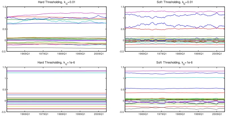
[image:13.595.106.502.164.372.2]Q= 1e-6
Figure 2. Posterior means of TVP-VAR(4) estimates from a typical three-variable system on prices, output and interest rate. In this case we want to assess the effect
of smaller values ofkQ on the posterior mean of the TVP-VAR coefficientsβt. The analysis above is based on a default prior for V (noninformative), which allows us to evaluate the effect of the soft and hard thresholding priors on Q. Similar analysis can be implemented for prior selection for V, in the case this parameter follows the subjective and objective Minnesota priors in equations (11) and (12), respectively. For instance, tighter choice of hyperparameters on the subjective and objective Minnesota priors forVwould not only result in shrinkage of βt towards time invariance (as it is the case in the bottom panel of Figure 2), but would also force coefficients to be exactly equal to zero and, thus, irrelevant for forecasting. For the sake of brevity such analysis is not implemented here. We rather focus in the next subsection on the ability of the different priors presented in this paper to prevent overparametrization and provide superior TVP-VAR forecasts.
3.2
Forecast evaluation
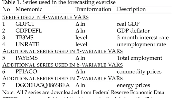
comparing TVP-VARs of different sizes we should be able to understand whether it is more important to consider nonlinearity in the VAR as opposed to adding more information by increasing the number of dependent variables. Table 1 describes all the variables used and how these define our four to seven-variable systems. We estimate all TVP-VARs in this section using data from 1960Q1, however, all variables in Table 1 are collected since 1948Q1 in order to be able to define a training sample 1948Q1-1959Q4 when using the Primiceri (2005) prior. Variables which are not already in rates are transformed into non-annualized quarter-on-quarter growth rates by taking first log-differences multiplied by 100. Monthly variables are transformed to quarterly by taking their average over the quarter.
Table 1. Series used in the forecasting exercise
No Mnemonic Tranformation Description
SERIES USED IN4-VARIABLEVARS
1 GDPC1 ∆ln real GDP
2 GDPDEFL ∆ln GDP deflator
3 TB3MS level 3-month interest rate
4 UNRATE level unemployment rate
ADDITIONAL SERIES USED IN5-VARIABLEVARS
5 PAYEMS ∆ln Total employment
ADDITIONAL SERIES USED IN6-VARIABLEVARS
6 PPIACO ∆ln commodity prices
ADDITIONAL SERIES USED IN7-VARIABLEVARS
7 DGOERA3Q086SBEA ∆ln energy prices
Note: All 7 series are downloaded from Federal Reserve Economic Data (FRED), and are available at http://research.stlouisfed.org/fred2/.
We estimate several TVP-VARs recursively over the period 1960Q1-2013Q2. All models have four lags and an intercept. In particular, we consider the following prior specifications which define our forecasting TVP-VARs:
1. Training sample prior: We use the original TVP-VAR whereβ0 N(βOLS,VOLS), and Q iW k+2,k2Q VOLS where βOLS and VOLS are the mean and variance of the OLS estimates from a time-invariant VAR estimated over the sample 1948Q1-1959Q4.
2. Traditional Minnesota prior: We use the original TVP-VAR where β0
N(βMI N,VMI N), and Q iW k+2,k2Q VMI N where βMI N and VMI N
are prior hyperparameters of the Minnesota prior (see appendix for exact definition).
3. Soft thresholding: Here we use the reparametrized TVP-VAR and we define
different ways to define a prior for V, i.e. noninformative (NI), subjective Minnesota (SM), and objective Minnesota priors (OM); see equations (10) -(12).
4. Hard thresholding: Here we use the reparametrized TVP-VAR and we define
Qii iG 1+2,kQ Vii , i =1, ...,m, whereV = diag(τ1, ...,τm). We allow for three different ways to define a prior forV, i.e. noninformative, subjective Minnesota, and objective Minnesota priors; see equations (10) - (12).
Subsequently, we have in total one TVP-VAR with training sample, one with Minnesota prior, three with hard thresholding, and three with soft thresholding. We also have models with four, five, six, and seven variables. This gives a total of 32 TVP-VARs to be evaluated in this forecasting exercise.
All prior hyperparameters for the time-varying coefficients and covariances used in this forecasting exercise are described in detail in the appendix. Note that selection ofkQ is of paramount importance for all four models in 1-4. In an ideal world selection of kQ could be based on a grid search, where the optimal value could be selected based on past forecast performance or insample fit (see Koop and Korobilis, 2013, for an illustration). However, when using MCMC such procedures have to be precluded from our analysis due to computational constraints. Therefore, and in order to avoid data-mining we set kQ = 0.01 for all TVP-VAR sizes even though in an ideal worldkQ should decrease as the TVP-VAR size increases; see again Koop and Korobilis (2013). While other choices ofkQ might give quite different forecasting results, given computational restrictions (this is the restriction that any applied economist estimating a TVP-VAR would face), the purpose of this exercise is to evaluate how different priors perform based on an arbitrary choice of prior hyperparameters. The insample results of the previous subsection suggest that the data-based priors proposed in this paper are more robust to suboptimal choices ofkQ, which is something that we should expect to verify out-of-sample.
We estimate the reparametrized TVP-VAR in equations (5) and (6). The original coefficient βt is recovered using the simple formula βt = α+αt, and forecasting at time t is implemented iteratively using the typical TVP-VAR specification in equations (3)-(4), by assuming for simplicity that the VAR parameters are the ones estimated at the last in-sample observation8, that is βt+hjt = βt, Ωt+hjt = Ωt. By
rearraging the elements of the parameter matrices, we can obtain the VAR in usual companion form as
yt =c+Byt 1+εt
8This is a simplifying assumption done in the literature with TVP-VAR models, whether they are
whereyt = y0t, ...,y0t p+1
0
,εt = (ε0
t, 0, ..., 0)
0
,c = (c0t, 0, ..., 0)0and
B= B1,t...Bp 1,t Bp,t
In(p 1) 0n(p 1) n , Σ =
Σt 0n n(p 1)
0n(p 1) n(p 1) .
Iteratedh-step ahead forecasts can be obtained using the formula
Et(yt+h) =
∑
ih=01Bic+Bhyt 1 (13)The forecasting exercise is performed in pseudo real time. For the daily data, 60% of the observations are used to estimate the model initially, i.e. T0 = 0.7T,
and forecastsybT0+hjT0 are calculated for h = 1, 4 and 8 quarters ahead. Then one quarterly observation is added and the sample becomesT1 = T0+1, each model
is re-estimated, and the coefficients βT1 are used in order to obtain the forecasts of ybT0+1+hjT0+1. This is done until the whole sample is exhausted, i.e. when
Tn = T. Notice that evaluating forecasts using only 40% of the sample is not an ideal situation, however, one has to consider the computational demands of estimating TVP-VARs of that size. Additionally, the out-of-sample period includes the turbulent ’00s where forecasting episodes, such as the Great Recession, are of extreme interest to policy-makers.
The results are evaluated using the Mean Squared Forecast Error (MSFE)9. When forecasting variableiat horizonh, these statistics are defined as
MSFEi,h = 1
n h
T h
∑
t=T0
b
yi,t+hjt yoi,t+h 2
where yoi,t+h are the observed out-of-sample values of yi,t+h. The MSFE statistic is presented relative to a benchmark 4-variable VAR(4) with constant coefficients estimated using least squares, so that values higher (lower) than one signify worse (better) performance of a specific TVP-VAR model compared to the VAR(4). Eval-uation of the relative MSFE is based only on the four variables which are common in all TVP-VARs, namely real GDP growth (GDPC1), price inflation (GDPDEFL), short-term interest rate (TB3MS), and the unemployment rate (UNRATE).
9It is interesting to note here that according to other metrics which evaluate the whole
Table 2. Relative MSFE of TVP-VAR models with various priors
GDPC1 GDPDEFL TB3MS UNRATE
h=1 h=4 h=8 h=1 h=4 h=8 h=1 h=4 h=8 h=1 h=4 h=8
VAR(4) 0.624 0.768 0.729 0.057 0.126 0.166 0.227 1.916 5.315 0.087 1.378 3.941
4-variable TVP-VARs:
h=1 h=4 h=8 h=1 h=4 h=8 h=1 h=4 h=8 h=1 h=4 h=8
TS 1.06 1.50 4.06 0.77 0.81 1.01 0.89 1.31 1.86 0.75 1.53 4.56
Minnesota 0.97 1.17 1.69 0.76 0.59 0.63 0.90 1.29 1.51 0.70 1.13 1.87
SOFTTHRESHOLDING
NI 0.91 1.33 1.82 0.70 0.95 1.72 0.63 1.01 1.41 0.72 1.10 2.09
SM 0.91 1.04 1.15 0.84 0.85 1.05 0.63 1.06 1.29 0.66 1.07 1.90
OM 0.91 1.02 1.16 0.80 0.75 1.02 0.60 1.05 1.18 0.60 1.03 1.71
HARDTHRESHOLDING
NI 0.87 1.23 1.77 0.72 0.76 0.85 0.85 1.44 1.85 0.66 1.06 2.29
SM 0.87 1.45 2.85 0.73 0.71 0.96 0.86 1.36 1.85 0.59 1.34 3.74
OM 0.88 1.20 1.66 0.67 0.55 0.74 0.87 1.18 1.51 0.48 1.12 2.59
5-variable TVP-VARs:
h=1 h=4 h=8 h=1 h=4 h=8 h=1 h=4 h=8 h=1 h=4 h=8
TS 0.93 1.65 3.88 0.89 0.65 0.69 0.92 1.55 2.07 0.76 1.71 4.62
Minnesota 0.98 1.36 3.08 0.79 0.76 0.77 0.91 1.64 2.34 0.79 1.83 4.95
SOFTTHRESHOLDING
NI 0.96 1.14 1.66 0.70 0.66 0.83 0.68 1.27 1.67 0.58 0.97 2.03
SM 0.82 1.28 1.98 0.83 0.64 0.71 0.79 1.35 1.79 0.46 1.12 2.75
OM 0.76 1.18 1.73 0.76 0.65 0.73 0.79 1.28 1.73 0.42 1.03 2.36
HARDTHRESHOLDING
NI 0.85 1.41 2.26 0.89 0.82 0.94 0.65 1.05 1.46 0.70 0.98 1.82
SM 0.85 1.24 2.46 0.71 0.60 0.85 0.81 1.53 2.36 0.63 1.32 3.95
Table 2. continued
GDPC1 GDPDEFL TB3MS UNRATE
6-variable TVP-VARs:
h=1 h=4 h=8 h=1 h=4 h=8 h=1 h=4 h=8 h=1 h=4 h=8
TS 1.31 1.34 1.51 1.81 0.89 1.41 1.15 1.32 1.35 1.33 1.02 1.60
Minnesota 1.22 1.17 1.15 1.33 0.62 0.89 1.10 1.26 1.24 1.68 1.23 2.98
SOFTTHRESHOLDING
NI 1.01 1.07 1.35 1.55 0.61 0.82 0.89 1.16 1.44 0.69 0.99 1.57
SM 0.89 0.99 0.97 1.03 0.72 0.74 0.99 1.19 1.37 1.00 0.99 1.59
OM 0.90 0.99 0.85 0.72 0.63 0.76 0.92 1.15 1.40 0.80 0.96 1.58
HARDTHRESHOLDING
NI 0.95 0.98 0.96 0.82 0.55 0.75 0.59 0.96 1.20 0.87 1.13 1.92
SM 1.02 1.37 1.81 1.43 0.85 1.01 1.41 1.89 2.33 0.73 0.83 1.84
OM 0.92 0.59 0.86 0.37 0.68 0.87 0.82 1.41 1.76 0.78 0.95 1.87
7-variable TVP-VARs:
h=1 h=4 h=8 h=1 h=4 h=8 h=1 h=4 h=8 h=1 h=4 h=8
TS 1.27 1.64 1.66 1.07 0.89 1.08 1.55 1.36 1.34 1.38 1.21 2.59
Minnesota 1.23 1.71 1.30 1.79 0.87 0.71 1.09 1.21 1.25 0.67 1.03 3.14
SOFTTHRESHOLDING
NI 1.19 1.36 1.40 1.01 0.55 0.55 0.65 0.97 1.35 0.58 0.60 0.99
SM 0.82 1.05 0.92 1.06 0.81 0.93 1.06 1.08 1.13 0.83 0.89 1.57
OM 0.81 0.98 0.94 0.64 0.61 0.50 1.03 0.97 1.17 0.50 0.69 1.21
HARDTHRESHOLDING
NI 1.03 1.02 1.02 1.13 0.59 0.73 0.95 1.18 1.39 0.82 0.85 1.24
SM 0.91 1.09 0.96 1.20 0.66 1.09 1.36 1.47 1.39 0.86 0.82 1.49
OM 0.90 1.05 0.92 0.86 0.59 0.87 1.08 1.32 1.35 0.80 0.63 1.36
Table entries for the 4-variable VAR(4) model with OLS are absolute MSFE values. For all other models ratios of MSFEs relative to the one for the VAR(4) are reported. Values higher than one signify worse
performance compared to the base VAR(4) model. Variable mnemonics are the ones defined in the main text, and follow Federal Reserve Economic Data (FRED).
Table 2 presents the results of this forecasting exercise. There are several stylized facts we can establish from such a table. First, TVP-VAR models improve massively upon simple VARs in forecasts of inflation at all horizons. There is also improvement in short-run forecasts of GDP and unemployment, implying that there are some nonlinearities in the short-run while we are better off in the long-run with the simple linear VAR model. For the short-term interest rate the VAR model seems to be hard to beat at all horizons. These results also comply with the findings of Korobilis (2013c) for UK data.
Second, while in constant parameter VARs we expect larger systems with more information to perform well, when considering nonlinearities in the form of time-varying coefficients and stochastic volatility there is no evidence that larger VAR models are better than smaller VAR models. There are two interpretations to this result. On the one hand, nonlinearities captured by the TVP-VAR might be the main reason for forecast improvement over the simple VAR(4) estimated with OLS. Therefore, larger systems add little to the forecasting ability of a smaller TVP-VAR. On the other hand, one can argue that larger TVP-VARs have the potential of improving upon smaller TVP-VARs conditional on achieving the right amount of shrinkage. In this paper, due to computational constrains we have used “default” prior hyperparameters for all VAR sizes, while careful application of shrinkage would require us to estimate the optimal shrinkage hyperparameter,kQ, for each VAR size. Koop and Korobilis (2013) implement such an approach, however, estimation of their TVP-VARs is based on fast and efficient approximations and not computationally expensive MCMC methods.
4
Conclusions
We have presented a framework for dealing efficiently with concerns of overfitting and overparametrization in time-varying parameter VARs. By means of data-based shrinkage priors we have managed to reduce the huge parameter space associated with coefficients which change value each time period, whilst at the same time computation has remained simple and feasible. We have examined several prior specifications which address varying needs for shrinkage in VAR models. Therefore, this paper has proposed an integrated treatment of TVP-VARs with automatic prior choices that are updated from the likelihood (data). Additionally, the algorithms presented here add minimal computation time to existing MCMC algorithms and result in improved numerical stability (through shrinkage we can prevent time-varying coefficients from exploding, and associated covariance matrices from becoming non-invertible).
References
[1] Belmonte, M. A. G., Koop, G. and Korobilis, D. (2014). Hierarchical shrinkage in time-varying parameter models. Journal of Forecasting, forthcoming.
[2] Bhattacharya, A. and Dunson, D. B. (2011). Sparse Bayesian infinite factor models. Biometrika 98, pp. 291-306.
[3] Bouriga, M. and Féron, O. (2013). Estimation of covariance matrices based on hierarchical inverse-Wishart priors. Journal of Statistical Planning and Inference 143, pp. 795-808.
[4] Chen, Z. and Dunson, D. (2003). Random effects selection in linear mixed models. Biometrics 59 (4), pp. 762-769.
[5] Clark, T. and Ravazzolo, F. (forthcoming). The macroeconomic forecasting performance of autoregressive models with alternative specifications of time-varying volatility. Journal of Applied Econometrics.
[6] Cooley, T. F. (1971). Estimation in the presence of sequential parameter varia-tion. Ph.D Thesis. Department of Economics, University of Pennsylvania.
[7] D’Agostino, A., Gambetti, L. and Giannone, D. (2013). Macroeconomic forecasting and structural change. Journal of Applied Econometrics 28, pp. 82-101.
[8] Doan, T., Litterman, R. and Sims, C. (1984). Forecasting and conditional projection using realistic prior distributions. Econometric Reviews, 3, pp. 1-100.
[9] Eisenstat, E., Chan, J. C. C. and Strachan, R. (2013). Stochastic model specifi-cation search for time-varying parameter VARs. manuscript.
[10] Frühwirth-Schnatter, S. and Wagner, H. (2010). Stochastic model specification search for Gaussian and partial non-Gaussian state space models. Journal of Econometrics 154, pp. 85–100.
[11] Giannone, D., Lenza, M. and Primiceri, G. E. (2012). Prior selection for vector autoregressions. Working Paper Series 1494, European Central Bank.
[12] Groen, J. J. J., Paap, R. and Ravazzolo, F. (2012). Real-time inflation forecasting in a changing world. Journal of Business and Economic Statistics, 31, pp. 29-44.
[14] Koop, G. and Korobilis, D. (2013). Large Time-Varying Parameter VARs. Journal of Econometrics 177, pp. 185-198.
[15] Korobilis, D. (2013a). Bayesian forecasting with highly correlated predictors. Economics Letters 118, pp. 148-150.
[16] Korobilis, D. (2013b). Hierarchical shrinkage priors for dynamic regressions with many predictors. International Journal of Forecasting 29, pp. 43-59.
[17] Korobilis, D. (2013c). VAR forecasting using Bayesian variable selection. Journal of Applied Econometrics 28, pp. 204-230.
[18] Kulhavý, R. and Zarrop, M. B. (1993). On a general concept of forgetting. International Journal of Control 58, pp. 905-924.
[19] Litterman, R. (1979). Techniques of forecasting using vector autoregressions. Federal Reserve Bank of Minneapolis Working Paper 115.
[20] Sims, C. (1989). A nine variable probabilistic macroeconomic forecasting model. Federal Reserve Bank of Minneapolis Discussion paper no. 14.
A
Technical Appendix
A.1
A Gibbs sampler for the TVP-VAR with data-based priors
In this Appendix we describe the hierarchical shrinkage priors for time-varying parameter VARs, and the associated modifications in the Markov Chain Monte Carlo (MCMC) algorithm which are needed in order to sample from the posterior distributions of all parameters. Consider the noncentered parametrization of the VAR
yt = z0tα+z0tαt+εt, (A.1)
αt = αt 1+ηt, (A.2)
subject to the initial condition α0 N(0, 0) δα(0), with δα(0) denoting the
Dirac delta function for coefficientα which is concetrated at zero. In this case the original coefficient βt can be recovered as βt = α+αt = β0+αt, that is we have effectively split the original coefficient into a “initial condition part” and a “time-varying part”.
We use the following prior on thek 1 vectorα:
α N(0,V),
V = diag(τ1, ...,τm),
τi
(
=2, for intercepts
iG κ1, 1 r12 , for coefficients onr-th lag ,
fori = 1, ...,k. The prior variance ofα = β0 is determined by the matrix V with diagonal element τi, where each diagonal element is defined to have an inverse-gamma prior10. The specific inverse-gamma prior is set-up in order to favour more shrinkage as the number of lags increases.
We define two cases of shrinkage priors forQ(note: Qis the variance ofηt). In the hard thresholding case we use
Qii iG 8, 1
r2 τ2i , and in the soft thresholding case we use
Q iW(k+1, 1e 3 V).
For the VAR covariance matrix Ωt we follow Primiceri (2005) and define the decomposition
Ωt =Lt 1DtD0tLt 10,
10Note that the noninformative prior in equation (10) can be obtained in the limit using an
where Lt is a lower triangular matrix with ones on the main diagonal, and Dt is a diagonal matrix. Denote by lt the n(n 1)/2 vector of non-zero and non-one elements of Lt, and by dt the vector consisting of all n diagonal elements in Dt. Then time variation inlt anddtis of the form
lt = lt 1+vt, logdt = logdt 1+wt,
wherevt N(0,S)andwt N(0,W). Given draws ofαandαt, it is easy to show that the posterior conditional distributions for lt and logdt are exactly the ones given in the appendix of Primiceri (2005); see also Koop and Korobilis (2010). Now it suffices to show that for the initial condition on lt and dt we set the relatively noninformative values
l0 N 0, 10 In(n 1)/2 ,
logd0 N(0, 10 In). Finally, the state covariancesSandW have priors
Sj iW j+1, 0.01 Ij ,
Wi,i iG(8, 0.1),
for j = 1, ...,n 1 and i = 1, ...,n, where the reader should note that S is block-diagonal and W is diagonal for estimation reasons; once again the appendix of Primiceri (2005) gives the exact details.
The conditional posteriors11 of all coefficients are:
1. Sampleαfrom
αj N α,Vα ,
where α = Vα ∑
t zt
Ω 1
t yt , Vα = V+∑
t zt
Ω 1
t zt , V = diag(τ1,...,τm) and yt =yt z0tαt.
2. Sampleτi(only for thoseithat do not refer to intercept coefficients) from
τij iG(ρ1i,ρ2i),
where ρ1i = 0.5+κ1, and ρ2i = 0.5 (αi)2+κ2. When using the Jeffrey’s
noninformative prior on τi then the posterior has the same form with the exception thatκ1 =κ2 =0. When using the data-based Minnesota prior then
see the next subsection.
11Here we use notation whereθj is the conditional posterior distribution ofθconditional on
3. Sample αtj using Carter and Kohn (1994) with initial condition α0
N(0, 0)and data(yet,zt)whereyet =yt z0tα.
4. Sample Qj using standard expressions from Inverse Wishart (or inverse Gamma, in the case of hard thresholding) posteriors; see Koop (2003).
5. Sample the covariance matrix conditional on all other parameters as in Primiceri (2005). To see that there are no differences, once we have draws of
αtandαwe can obtain a draw ofβt simply by using the identityβt =α+αt, in which case we can estimate Ωt using the original TVP-VAR in equations
(3) and (4).
A.2
Sampling of
τ
iunder the data-based Minnesota prior
When using the data-based Minnesota prior we just have to sample a few more hyper-parameters we have introduced from their conditional posteriors. We remind that the full prior is of the form
α N(0,V),
V = diag(τ1, ...,τm),
τi = λi 1ξir1, r =1, ...,p
λi 1 G(v/2,v/2),
ξr =
∏
rl=1δl,δ1 G(ρ1, 1),
δl G(ρ2, 1), l 2 .
Step 1 of the Gibbs sampler algorithm presented above (sampling ofαconditional on τi) is not affected by the new hierarchical layers we have added in order to sampleτi. What we need to adapt is Step 2 which now becomes
2*. (a) Sampleλ 1from
λi 1j Ga v+1
2 ,
v+ξrα2i
2 !
.
(b) Sample δ1from
δ1j G ρ1+m 2, 1+
1 2
" p
∑
r=1 ξ(r1)
n2
∑
j=1
λjr1α2jr
where α2r = α21r, ...,α2n2r denotes the n2 elements of α which corre-spond to coefficients on ther-th VAR lag,r=1, ...,p, andξr(1) =∏rc=2δc (c) Sample δl forl 2 from
δlj G ρ2+n n
2 (r l+1), 1+ 1 2
" p
∑
r=1 ξ(rl)
n2
∑
j=1
λjr1α2jr
!#! ,
whereξ(rl) =∏rc=1,c6=lδc
For more details the reader is referred to Bhattacharya and Dunson (2011), who developed this shrinkage prior for the case of a factor model with unkown number of factors.
A.3
The traditional Minnesota (Litterman, 1979) prior
One of the benchmark priors used in this paper, other than the training sample prior of Primiceri (2005), is the traditional Minnesota prior of Litterman (1979) adapted for the time-varying parameter VAR. This adaption of the Minnesota prior is not new, since very early Doan, Litterman and Sims (1984) have shown how the Minnesota prior can provide shrinkage both in constant parameter and time-varying parameter VARs. We apply the Minnesota prior in the original TVP-VAR12 of equations (3)-(4). The prior takes the following form
β N(b,V),
wherebis one for coefficients on the first own lag, and zero otherwise, and
Vij =
8 > < > :
100s2i if intercept
λ/r2 ifi =j
λ s2i
r2s2
l
ifi6=j
(A.3)
forr = 1, ...,p, i = 1, ...,n,and j = 1, ...,k with k = np+1. Here s2i is the residual variance from the unrestricted p-lag univariate autoregression for variable i. The degree of shrinkage depends on a single hyperparameterλwhich, for the purpose of computing the forecasts of the empirical section, we fix to 1.
12One can also apply the Minnesota prior in the equivalent reparametrized TVP-VAR in